Astigmatic polarized beamlets

Standard stigmatic beamlets are limited to symmetric systems. For the modeling of arbitrary optical systems, including off-axis components, tilted lenses, or complex media like atmospheric turbulence, the package provides the AstigmaticGaussianBeamlet. This type implements the astigmatic Gaussian beamlet ray tracing formalism initially proposed by Greynolds (1986) [13, 14].

However, this idea has been referred to in multiple ways over the last few decades, including but not limited to: Gaussian Beamlet Tracing (GBT), Fat Ray Tracing (FRT), Parabasal Ray Tracing (PRT), Complex Ray Tracing (CRT), Gauss Beamlet Propagation (GBP) and Beam Synthesis Propagation (BSP).

Formalism

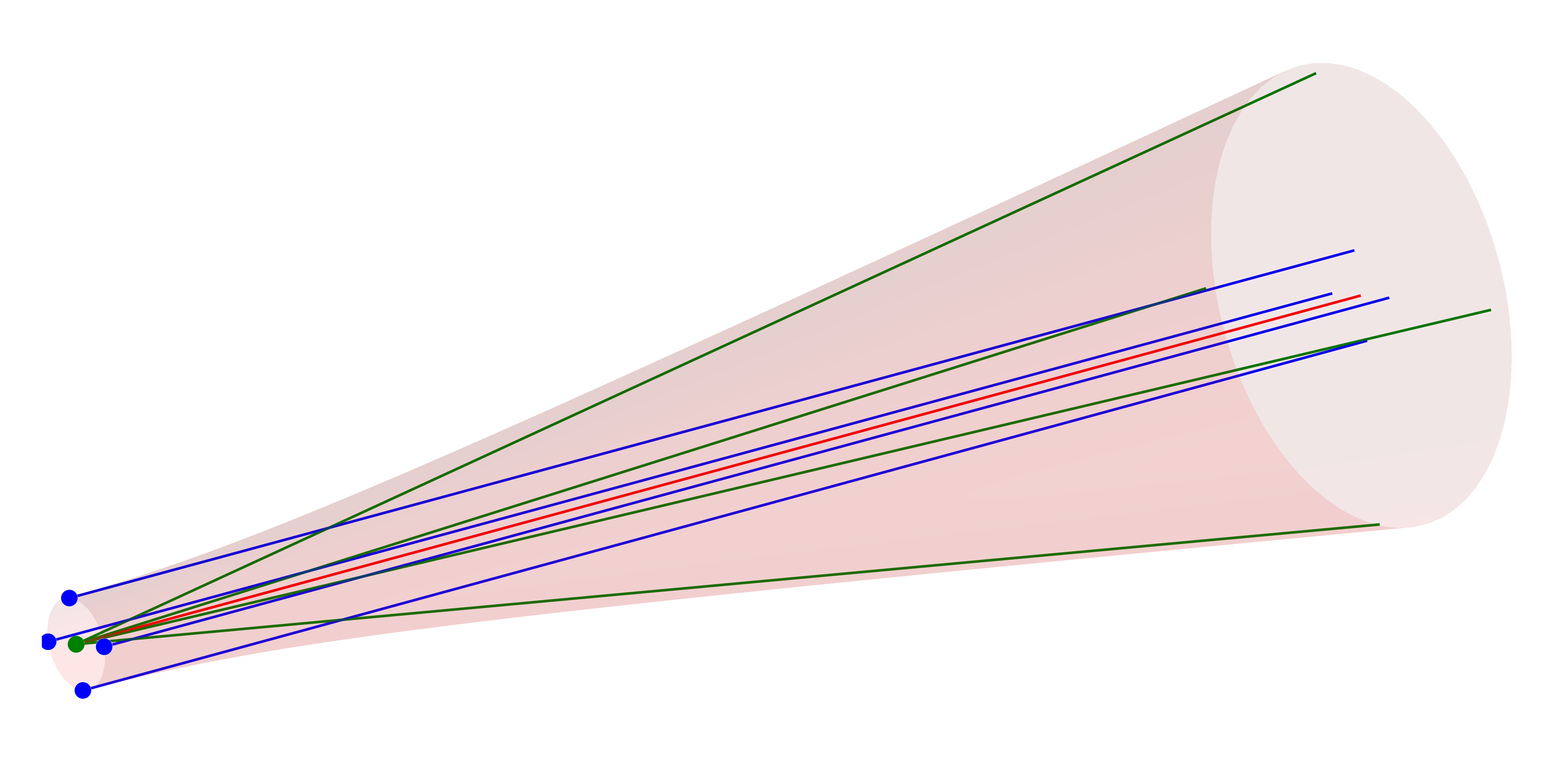
Similar to the Gauss model presented in the Stigmatic beamlets chapter, an astigmatic beamlet can represented by a cluster of 9 rays:

These rays can be thought of tracking the complex curvature matrix $\mathbf{Q}(z)$ through the system. The key assumptions made in order for this formalism to hold are:

The initial ordering of the geometric beams/rays is shown in the figure below. The colors represent the chief (red), waist (blue) and divergence (green) beams.

As with the GaussianBeamlet, tracing these rays through a system allows the reconstruction of the waist envelope and electric field. The reduced complex amplitude of the Gaussian beamlet is computed as

\[\psi(\mathbf{r}) = \frac{E_0}{\sqrt{\mathbf{h}_1 \times \mathbf{h}_2}} \cdot \exp \left( i k \frac{(\mathbf{h}_1 \times \mathbf{r})(\mathbf{u}_2 \cdot \mathbf{r}) - (\mathbf{h}_2 \times \mathbf{r})(\mathbf{u}_1 \cdot \mathbf{r})}{2 \mathbf{h}_1 \times \mathbf{h}_2} \right) \,,\]

where $\mathbf{h}_{1,2}$ and $\mathbf{u}_{1,2}$ are the two-dimensional complex ray height and angle vectors on the plane perpendicular to the chief ray [13, 15, 16]. By also tracing a 3D-field vector along the chief ray based on the formalism introduced in the Polarized rays section, polarization effects can be considered when calculating $\psi$ [17]. For a simple lens setup, the resulting waist is illustrated in the image below.

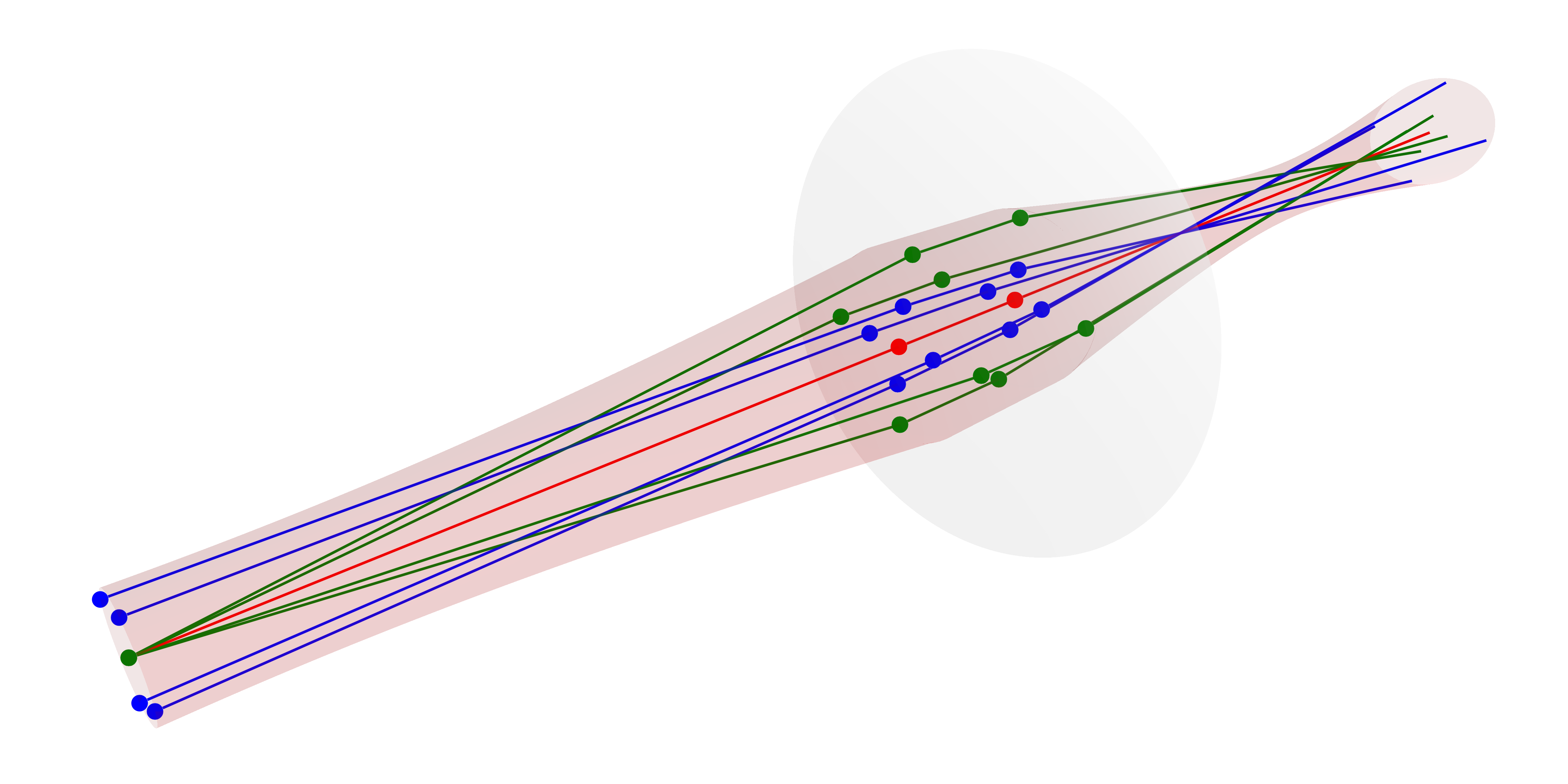
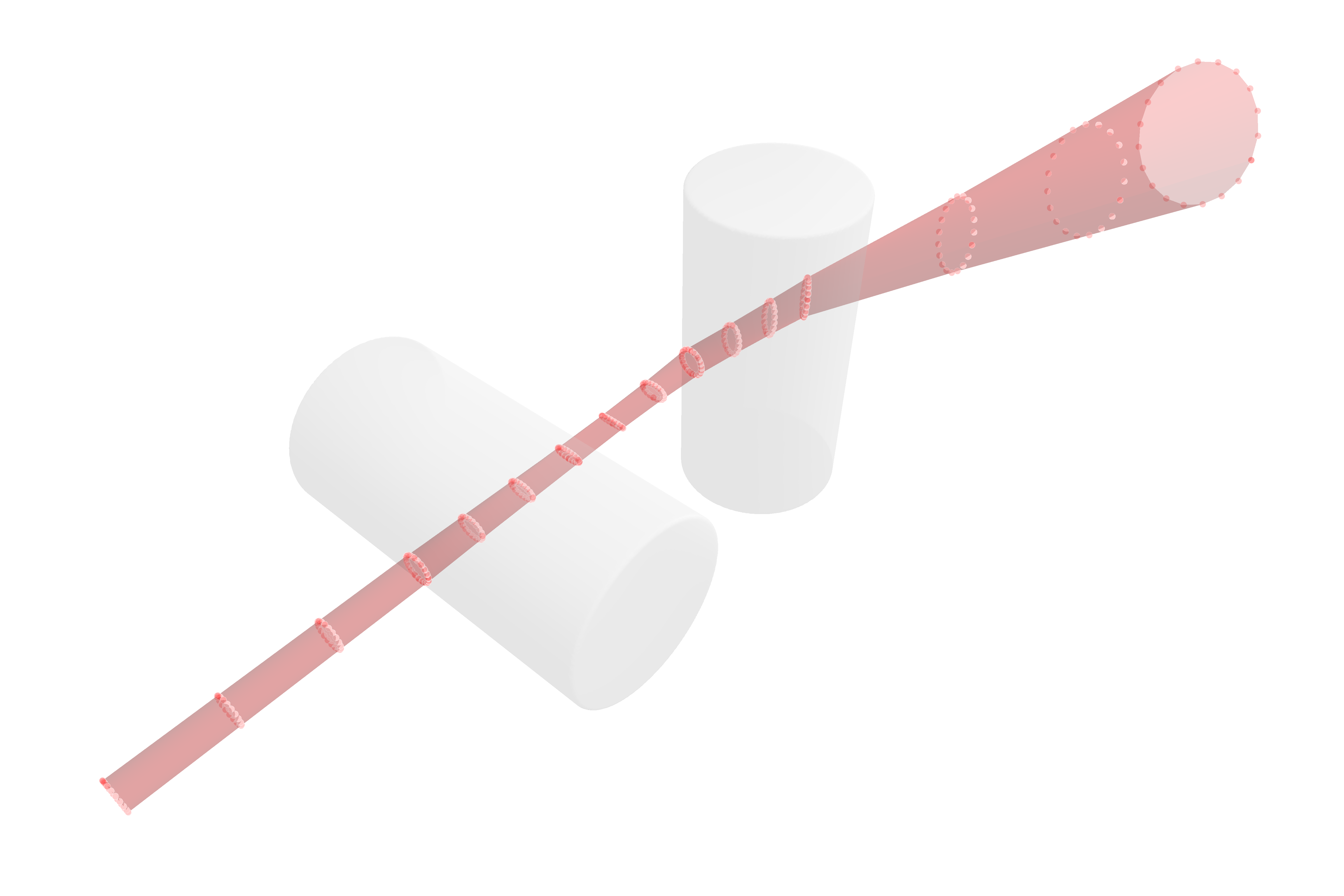
While the above beam closely matches the example Gaussian given in the previous section (Obtaining the beam parameters), the real advantage of this extended method lies in the tracing of non-symmetric systems. For a tilted two cylinder lens system, the following result with strong astigmatic effects is obtained. Multiple waist slices are marked with red dots.

The phase factor due to the optical path length of the central ray ($e^{i k (z + \Delta L)}$) is added to the reduced field $\psi$ during the final field calculation for each beamlet. More information on the mathemathics behind this formalism can be found below in The Curvature Matrix $\mathbf{Q}$ section.

Astigmatic beamlets

You can construct a single astigmatic beamlet with a specified waist and polarization:

AstigmaticGaussianBeamlet(position, direction, λ, w0; kwargs...)

The constructor will spawn an AstigmaticGaussianBeamlet which is implemented as follows:

AstigmaticGaussianBeamlet{T} <: AbstractBeam{T, PolarizedRay{T}}

Calculating astigmatic beam parameters

To obtain the physical vector electric field [V/m] at any point:

# Field at world position (x, y, z)
E_vec = polarized_field(agb, [0.01, 0, 0], 10.0)

# Decompose a field from a detector into a new AstigmaticBeamGroup
beams = WavefrontBeamletDecomposition(x, z, amplitude, phase, dir, λ)

# Solve system (propagate all beamlets to next segment)
solve_system!(system, beams)

The Curvature Matrix $\mathbf{Q}$

The relationship between the auxiliary rays and the complex curvature of the beam is defined by the matrix equation $\mathbf{Q} = \mathbf{U}\mathbf{H}^{-1}$. By arranging the transverse components of the complex rays into $2 \times 2$ matrices $\mathbf{H} = [\mathbf{h}_1, \mathbf{h}_2]$ and $\mathbf{U} = [\mathbf{u}_1, \mathbf{u}_2]$, we can solve for the individual components of $\mathbf{Q}$:

\[\mathbf{Q} = \frac{1}{\mathbf{h}_1 \times \mathbf{h}_2} \begin{bmatrix} u_{1x} h_{2y} - u_{2x} h_{1y} & u_{2x} h_{1x} - u_{1x} h_{2x} \\ u_{1y} h_{2y} - u_{2y} h_{1y} & u_{2y} h_{1x} - u_{1y} h_{2x} \end{bmatrix}\]

The diagonal elements $Q_{xx}$ and $Q_{yy}$ describe the phase curvature (and beam width) along the primary axes, while the off-diagonal elements $Q_{xy}$ (which must equal $Q_{yx}$ for a paraxial beam) describe the general astigmatism or twist of the wavefront. This representation allows the formalism to track complex, rotating beam profiles as they propagate through non-orthogonal optical systems. It is important to note that this matrix is not directly tracked during beamlet propagation in BMO. More information can be found in the works of Kochkina (2013) and Ashcraft et al. (2024) [18, 19].

Physical Beam Cross-Section

While the complex curvature matrix $\mathbf{Q}$ determines the phase and amplitude of the field, extracting the physical $1/e^2$ irradiance footprint (the principal axes of the beam ellipse) requires calculating the spot covariance matrix. This relates directly to the internal code of the waist_parameters function.

As explicitly modeled for general astigmatic Gaussian beams [20], the matrix describing this intensity ellipse is directly derived from $\operatorname{Im}(\mathbf{Q})$. The eigendecomposition of this matrix (or its inverse) yields eigenvalues that correspond exactly to the squared physical semi-axes of the beam.

The spatial spot matrix $\mathbf{S}$, which describes the boundary of this intensity ellipse, is proportional to $\operatorname{Im}(\mathbf{Q})^{-1}$. A fundamental property of Hamiltonian optics (the symplectic invariant) dictates that for any physically valid, non-twisted Gaussian beam, the imaginary part of the curvature matrix satisfies:

\[\operatorname{Im}(\mathbf{Q}) = (\mathbf{H} \mathbf{H}^\dagger)^{-1}\]

This identity implies that the spatial spot covariance matrix $\mathbf{S}$, which defines the beam envelope, is directly proportional to the outer product of the complex ray height matrix: $\mathbf{S} \propto \mathbf{H} \mathbf{H}^\dagger$.

In BeamletOptics, this calculation is mapped directly to the 3D global coordinate system. Using the two complex 3D ray vectors $\mathbf{h}_1$ and $\mathbf{h}_2$, the $3 \times 3$ physical covariance matrix is formed by taking the real part of the tensor product:

\[\mathbf{S} = \operatorname{Re}(\mathbf{h}_1 \mathbf{h}_1^\dagger + \mathbf{h}_2 \mathbf{h}_2^\dagger)\]

Expanding the complex vectors into their real and imaginary parts ($\mathbf{h} = \mathbf{h}_r + i \mathbf{h}_i$), this is implemented as:

\[\mathbf{S} = \mathbf{h}_{1r} \mathbf{h}_{1r}^T + \mathbf{h}_{1i} \mathbf{h}_{1i}^T + \mathbf{h}_{2r} \mathbf{h}_{2r}^T + \mathbf{h}_{2i} \mathbf{h}_{2i}^T\]

To find the true physical principal axes of the general astigmatic beam, the waist_parameters function computes the eigendecomposition of this symmetric matrix $\mathbf{S}$. The resulting eigenvectors provide the orientation, while the square roots of the eigenvalues provide the lengths of the orthogonal major and minor 3D semi-axes. This approach ensures an objective and stable definition of the intensity footprint, even in systems where the beam undergoes rapid rotation, skew, or non-orthogonal transformations [8, 17, 20].