Examples

These are some basic examples of use of the package:

julia> using Measurements
julia> a = measurement(4.5, 0.1)4.5 ± 0.1
julia> b = 3.8 ± 0.43.8 ± 0.4
julia> 2a + b12.8 ± 0.45
julia> a - 1.2b-0.06 ± 0.49
julia> l = measurement(0.936, 1e-3);
julia> T = 1.942 ± 4e-3;
julia> g = 4pi^2*l/T^29.798 ± 0.042
julia> c = measurement(4)4.0 ± 0.0
julia> a*c18.0 ± 0.4
julia> sind(94 ± 1.2)0.9976 ± 0.0015
julia> x = 5.48 ± 0.67;
julia> y = 9.36 ± 1.02;
julia> log(2x^2 - 3.4y)3.34 ± 0.53
julia> atan(y, x)1.041 ± 0.071

Measurements from Strings

You can construct Measurement{Float64} objects from strings. Within parentheses there is the uncertainty referred to the corresponding last digits.

julia> using Measurements
julia> measurement("-12.34(56)")-12.34 ± 0.56
julia> measurement("+1234(56)e-2")12.34 ± 0.56
julia> measurement("123.4e-1 +- 0.056e1")12.34 ± 0.56
julia> measurement("(-1.234 ± 0.056)e1")-12.34 ± 0.56
julia> measurement("1234e-2 +/- 0.56e0")12.34 ± 0.56
julia> measurement("-1234e-2")-12.34 ± 0.0

It is also possible to use parse(Measurement{T}, string) to parse the string as a Measurement{T}, with T<:AbstractFloat. This has been tested with standard numeric floating types (Float16, Float32, Float64, and BigFloat).

julia> using Measurements
julia> parse(Measurement{Float16}, "19.5 ± 2.8")19.5 ± 2.8
julia> parse(Measurement{Float32}, "-7.6 ± 0.4")-7.6 ± 0.4
julia> parse(Measurement{Float64}, "4 ± 1.3")4.0 ± 1.3
julia> parse(Measurement{BigFloat}, "+5.1 ± 3.3")5.099999999999999999999999999999999999999999999999999999999999999999999999999986 ± 3.299999999999999999999999999999999999999999999999999999999999999999999999999993

Correlation Between Variables

Here you can see examples of how functionally correlated variables are treated within the package:

julia> using Measurements, SpecialFunctions
julia> x = 8.4 ± 0.78.4 ± 0.7
julia> x - x0.0 ± 0.0
julia> x/x1.0 ± 0.0
julia> x*x*x - x^30.0 ± 0.0
julia> sin(x)/cos(x) - tan(x) # They are equal within numerical accuracy-2.220446049250313e-16 ± 0.0
julia> y = -5.9 ± 0.2;
julia> beta(x, y) - gamma(x)*gamma(y)/gamma(x + y)2.8e-14 ± 4.0e-14

You will get similar results for a variable that is a function of an already existing Measurement object:

julia> using Measurements
julia> x = 8.4 ± 0.7;
julia> u = 2x;
julia> (x + x) - u0.0 ± 0.0
julia> u/2x1.0 ± 0.0
julia> u^3 - 8x^30.0 ± 0.0
julia> cos(x)^2 - (1 + cos(u))/20.0 ± 0.0

A variable that has the same nominal value and uncertainty as u above but is not functionally correlated with x will give different outcomes:

julia> using Measurements
julia> x = 8.4 ± 0.7;
julia> v = 16.8 ± 1.4;
julia> (x + x) - v0.0 ± 2.0
julia> v / 2x1.0 ± 0.12
julia> v^3 - 8x^30.0 ± 1700.0
julia> cos(x)^2 - (1 + cos(v))/20.0 ± 0.88

@uncertain Macro

Macro @uncertain can be used to propagate uncertainty in arbitrary real or complex functions of real arguments, including functions not natively supported by this package.

julia> using Measurements, SpecialFunctions
julia> @uncertain (x -> complex(zeta(x), exp(eta(x)^2)))(2 ± 0.13)(1.64 ± 0.12) + (1.967 ± 0.043)im
julia> @uncertain log(9.4 ± 1.3, 58.8 ± 3.7)1.82 ± 0.12
julia> log(9.4 ± 1.3, 58.8 ± 3.7) # Exact result1.82 ± 0.12
julia> @uncertain atan(10, 13.5 ± 0.8)0.638 ± 0.028
julia> atan(10, 13.5 ± 0.8) # Exact result0.638 ± 0.028

You usually do not need to define a wrapping function before using it. In the case where you have to define a function, like in the first line of previous examples, anonymous functions allow you to do it in a very concise way.

The macro works with functions calling C/Fortran functions as well. For example, Cuba.jl package performs numerical integration by wrapping the C Cuba library. You can define a function to numerically compute with Cuba.jl the integral defining the error function and pass it to @uncertain macro. Compare the result with that of the erf function, natively supported in Measurements.jl package

julia> using Measurements, Cuba, SpecialFunctions
julia> cubaerf(x::Real) =
           2x/sqrt(pi)*cuhre((t, f) -> f[1] = exp(-abs2(t[1]*x)))[1][1]cubaerf (generic function with 1 method)
julia> @uncertain cubaerf(0.5 ± 0.01)0.5205 ± 0.0088
julia> erf(0.5 ± 0.01) # Exact result0.5205 ± 0.0088

Also here you can use an anonymous function instead of defining the cubaerf function, do it as an exercise. Remember that if you want to numerically integrate a function that returns a Measurement object you can use QuadGK.jl package, which is written purely in Julia and in addition allows you to set Measurement objects as endpoints, see below.

julia> using Measurements, SpecialFunctions

julia> @uncertain zeta(13.4 ± 0.8) + eta(8.51 ± 0.67)
ERROR: MethodError: no method matching zeta(::Measurement{Float64})
[...]

julia> using Measurements, SpecialFunctions

julia> @uncertain(zeta(13.4 ± 0.8)) +  @uncertain(eta(8.51 ± 0.67))
1.9974 ± 0.0012

julia> using Measurements, SpecialFunctions

julia> @uncertain (x -> polygamma(0, x))(4.8 ± 0.2)
1.461 ± 0.046

julia> digamma(4.8 ± 0.2)   # Exact result
1.461 ± 0.046

Complex Measurements

Here are a few examples about uncertainty propagation of complex-valued measurements.

julia> using Measurements
julia> u = complex(32.7 ± 1.1, -3.1 ± 0.2);
julia> v = complex(7.6 ± 0.9, 53.2 ± 3.4);
julia> 2u + v(73.0 ± 2.4) + (47.0 ± 3.4)im
julia> sqrt(u * v)(33.0 ± 1.1) + (26.0 ± 1.1)im

You can also verify the Euler's formula

julia> using Measurements
julia> u = complex(32.7 ± 1.1, -3.1 ± 0.2);
julia> cis(u)(6.3 ± 23.0) + (21.3 ± 8.1)im
julia> cos(u) + sin(u)*im(6.3 ± 23.0) + (21.3 ± 8.1)im

Missing Measurements

Measurement objects are poisoned by missing values as expected:

julia> using Measurements
julia> x = -34.62 ± 0.93-34.62 ± 0.93
julia> y = missing ± 1.5missing
julia> x ^ 2 / ymissing

Arbitrary Precision Calculations

If you performed an exceptionally good experiment that gave you extremely precise results (that is, with very low relative error), you may want to use arbitrary precision (or multiple precision) calculations, in order not to loose significance of the experimental results. Luckily, Julia natively supports this type of arithmetic and so Measurements.jl does. You only have to create Measurement objects with nominal value and uncertainty of type BigFloat.

For example, you want to measure a quantity that is the product of two observables $a$ and $b$, and the expected value of the product is $12.00000007$. You measure $a = 3.00000001 \pm (1\times 10^{-17})$ and $b = 4.0000000100000001 \pm (1\times 10^{-17})$ and want to compute the standard score of the product with stdscore. Using the ability of Measurements.jl to perform arbitrary precision calculations you discover that

julia> using Measurements
julia> a = BigFloat("3.00000001") ± BigFloat("1e-17");
julia> b = BigFloat("4.0000000100000001") ± BigFloat("1e-17");
julia> stdscore(a * b, BigFloat("12.00000007"))7.999999997599999878080000420160000093695993825308195353920411656927305928530607

the measurement significantly differs from the expected value and you make a great discovery. Instead, if you used double precision accuracy, you would have wrongly found that your measurement is consistent with the expected value:

julia> using Measurements
julia> stdscore((3.00000001 ± 1e-17)*(4.0000000100000001 ± 1e-17), 12.00000007)0.0

and you would have missed an important prize due to the use of an incorrect arithmetic.

Of course, you can perform any mathematical operation supported in Measurements.jl using arbitrary precision arithmetic:

julia> using Measurements
julia> a = BigFloat("3.00000001") ± BigFloat("1e-17");
julia> b = BigFloat("4.0000000100000001") ± BigFloat("1e-17");
julia> hypot(a, b)5.000000014000000080000000000000000000000000000000000000000000000000000000000013 ± 9.999999999999999999999999999999999999999999999999999999999999999999999999999967e-18
julia> log(2a) ^ b10.30668110995484998100000000000000000000000000000000000000000000000000000000005 ± 9.699999999999999999999999999999999999999999999999999999999999999999999999999966e-17

Operations with Arrays and Linear Algebra

You can create arrays of Measurement objects and perform mathematical operations on them in the most natural way possible:

julia> using Measurements
julia> A = [1.03 ± 0.14, 2.88 ± 0.35, 5.46 ± 0.97]3-element Vector{Measurement{Float64}}:
 1.03 ± 0.14
 2.88 ± 0.35
 5.46 ± 0.97
julia> B = [0.92 ± 0.11, 3.14 ± 0.42, 4.67 ± 0.58]3-element Vector{Measurement{Float64}}:
 0.92 ± 0.11
 3.14 ± 0.42
 4.67 ± 0.58
julia> exp.(sqrt.(B)) .- log.(A)3-element Vector{Measurement{Float64}}:
 2.58 ± 0.2
 4.82 ± 0.71
  7.0 ± 1.2
julia> @. cos(A) ^ 2 + sin(A) ^ 23-element Vector{Measurement{Float64}}:
 1.0 ± 0.0
 1.0 ± 0.0
 1.0 ± 0.0

If you originally have separate arrays of values and uncertainties, you can create an array of Measurement objects using measurement or ± with the dot syntax for vectorizing functions:

julia> using Measurements, Statistics
julia> C = measurement.([174.9, 253.8, 626.3], [12.2, 19.4, 38.5])3-element Vector{Measurement{Float64}}:
 175.0 ± 12.0
 254.0 ± 19.0
 626.0 ± 38.0
julia> sum(C)1055.0 ± 45.0
julia> D = [549.4, 672.3, 528.5] .± [7.4, 9.6, 5.2]3-element Vector{Measurement{Float64}}:
 549.4 ± 7.4
 672.3 ± 9.6
 528.5 ± 5.2
julia> mean(D)583.4 ± 4.4

Some linear algebra functions work out-of-the-box, without defining specific methods for them. For example, you can solve linear systems, do matrix multiplication and dot product between vectors, find inverse, determinant, and trace of a matrix, do LU and QR factorization, etc. Additional linear algebra methods (eigvals, cholesky, etc.) are provided by GenericLinearAlgebra.jl.

julia> using Measurements, LinearAlgebra
julia> A = [(14 ± 0.1) (23 ± 0.2); (-12 ± 0.3) (24 ± 0.4)]2×2 Matrix{Measurement{Float64}}:
  14.0±0.1  23.0±0.2
 -12.0±0.3  24.0±0.4
julia> b = [(7 ± 0.5), (-13 ± 0.6)]2-element Vector{Measurement{Float64}}:
   7.0 ± 0.5
 -13.0 ± 0.6
julia> x = A \ b2-element Vector{Measurement{Float64}}:
 0.763 ± 0.031
 -0.16 ± 0.018
julia> A * x ≈ btrue
julia> dot(x, b)7.42 ± 0.6
julia> det(A)612.0 ± 9.5
julia> tr(A)38.0 ± 0.41
julia> A * inv(A) ≈ Matrix{eltype(A)}(I, size(A))true
julia> lu(A)LinearAlgebra.LU{Measurement{Float64}, Matrix{Measurement{Float64}}, Vector{Int64}}
L factor:
2×2 Matrix{Measurement{Float64}}:
    1.0±0.0    0.0±0.0
 -0.857±0.022  1.0±0.0
U factor:
2×2 Matrix{Measurement{Float64}}:
 14.0±0.1   23.0±0.2
  0.0±0.0  43.71±0.67
julia> qr(A)LinearAlgebra.QR{Measurement{Float64}, Matrix{Measurement{Float64}}, Vector{Measurement{Float64}}}
Q factor: 2×2 LinearAlgebra.QRPackedQ{Measurement{Float64}, Matrix{Measurement{Float64}}, Vector{Measurement{Float64}}}
R factor:
2×2 Matrix{Measurement{Float64}}:
 -18.44±0.21  -1.84±0.52
    0.0±0.0   33.19±0.33

Derivative, Gradient and Uncertainty Components

In order to propagate the uncertainties, Measurements.jl keeps track of the partial derivative of an expression with respect to all independent measurements from which the expression comes. The package provides a convenient function, Measurements.derivative, that returns the partial derivative of an expression with respect to independent measurements. Its vectorized version can be used to compute the gradient of an expression with respect to multiple independent measurements.

julia> using Measurements
julia> x = 98.1 ± 12.798.0 ± 13.0
julia> y = 105.4 ± 25.6105.0 ± 26.0
julia> z = 78.3 ± 14.178.0 ± 14.0
julia> Measurements.derivative(2x - 4y, x)2.0
julia> Measurements.derivative(2x - 4y, y)-4.0
julia> Measurements.derivative.(log1p(x) + y^2 - cos(x/y), [x, y, z])3-element Vector{Float64}:
   0.017700515090289737
 210.7929173496422
   0.0

The last result shows that the expression does not depend on z.

julia> w = y^(3//4)*log(y) + 3x - cos(y/x)
447.0410543780643 ± 52.41813324207829

julia> abs.(Measurements.derivative.(w, [x, y]) .* Measurements.uncertainty.([x, y]))
2-element Array{Float64,1}:
 37.9777
 36.1297

julia> vecnorm(Measurements.derivative.(w, [x, y]) .* Measurements.uncertainty.([x, y]))
52.41813324207829

julia> Measurements.uncertainty_components(w)
Dict{Tuple{Float64,Float64,Float64},Float64} with 2 entries:
  (98.1, 12.7, 0.303638)  => 37.9777
  (105.4, 25.6, 0.465695) => 36.1297

julia> norm(collect(values(Measurements.uncertainty_components(w))))
52.41813324207829

stdscore Function

You can get the distance in number of standard deviations between a measurement and its expected value (not a Measurement) using stdscore:

julia> using Measurements
julia> stdscore(1.3 ± 0.12, 1)2.5000000000000004

You can use the same function also to test the consistency of two measurements by computing the standard score between their difference and zero. This is what stdscore does when both arguments are Measurement objects:

julia> using Measurements
julia> stdscore((4.7 ± 0.58) - (5 ± 0.01), 0)-0.5171645175253433
julia> stdscore(4.7 ± 0.58, 5 ± 0.01)-0.5171645175253433

weightedmean Function

Calculate the weighted and arithmetic means of your set of measurements with weightedmean and mean respectively:

julia> using Measurements, Statistics
julia> weightedmean((3.1±0.32, 3.2±0.38, 3.5±0.61, 3.8±0.25))3.47 ± 0.17
julia> mean((3.1±0.32, 3.2±0.38, 3.5±0.61, 3.8±0.25))3.4 ± 0.21

Measurements.value and Measurements.uncertainty Functions

Use Measurements.value and Measurements.uncertainty to get the values and uncertainties of measurements. They work with real and complex measurements, scalars or arrays:

julia> using Measurements
julia> Measurements.value(94.5 ± 1.6)94.5
julia> Measurements.uncertainty(94.5 ± 1.6)1.6
julia> Measurements.value.([complex(87.3 ± 2.9, 64.3 ± 3.0), complex(55.1 ± 2.8, -19.1 ± 4.6)])2-element Vector{ComplexF64}:
 87.3 + 64.3im
 55.1 - 19.1im
julia> Measurements.uncertainty.([complex(87.3 ± 2.9, 64.3 ± 3.0), complex(55.1 ± 2.8, -19.1 ± 4.6)])2-element Vector{ComplexF64}:
 2.9 + 3.0im
 2.8 + 4.6im

Calculating the Covariance and Correlation Matrices

Calculate the covariance and correlation matrices of multiple Measurements with the functions Measurements.cov and Measurements.cor:

julia> using Measurements
julia> x = measurement(1.0, 0.1)1.0 ± 0.1
julia> y = -2x + 108.0 ± 0.2
julia> z = -3x-3.0 ± 0.3
julia> cov([x, y, z])ERROR: UndefVarError: `cov` not defined in `Main`
Suggestion: check for spelling errors or missing imports.
Hint: a global variable of this name also exists in Statistics.
julia> cor([x, y, z])ERROR: UndefVarError: `cor` not defined in `Main`
Suggestion: check for spelling errors or missing imports.
Hint: a global variable of this name also exists in Statistics.

Creating Correlated Measurements from their Nominal Values and a Covariance Matrix

Using Measurements.correlated_values, you can correlate the uncertainty of fit parameters given a covariance matrix from the fitted results. An example using LsqFit.jl:

julia> using Measurements, LsqFit
julia> @. model(x, p) = p[1] + x * p[2]model (generic function with 1 method)
julia> xdata = range(0, stop=10, length=20)0.0:0.5263157894736842:10.0
julia> ydata = model(xdata, [1.0 2.0]) .+ 0.01 .* randn.()20-element Vector{Float64}:
  1.0037919287247208
  2.063515188589258
  3.1044313850900243
  4.171650601634867
  5.202051609051918
  6.241095961719974
  7.3167101289950125
  8.369599875298801
  9.434196196299386
 10.466428878438817
 11.497770932033259
 12.58213875049429
 13.629370226186735
 14.683904174161954
 15.729371084346566
 16.78478634966386
 17.856926229344076
 18.888447921657363
 19.94753835444619
 20.989981590288924
julia> p0 = [0.5, 0.5]2-element Vector{Float64}:
 0.5
 0.5
julia> fit = curve_fit(model, xdata, ydata, p0)LsqFit.LsqFitResult{Vector{Float64}, Vector{Float64}, Matrix{Float64}, Vector{Float64}, Vector{LsqFit.LMState{LsqFit.LevenbergMarquardt}}}([1.001158463786253, 1.9994053809074022], [-0.0026334649384678332, -0.010038103272793641, 0.0013643217566521315, -0.013536273257979126, 0.008381340855181385, 0.021655609717337043, -0.0016399360274901298, -0.002211060801066367, -0.01448876027143875, 0.005597179119341433, 0.02657374705511195, -0.005475449875707028, -0.00038830403794243296, -0.0026036304829499812, 0.004248080862650383, 0.0011514370755669745, -0.018669821074436044, 0.0021271081424885097, -0.004644703116127857, 0.005230682571351508], [1.0000000000018918 0.0; 1.0000000000018918 0.5263157894772135; … ; 1.000000000075144 9.473684210516485; 1.000000000075144 10.000000000103736], true, Iter     Function value   Gradient norm
------   --------------   --------------
, Float64[])
julia> coeficients = Measurements.correlated_values(coef(fit), estimate_covar(fit))2-element Vector{Measurement{Float64}}:
  1.0012 ± 0.0048
 1.99941 ± 0.00082
julia> f(x) = model(x, coeficients)f (generic function with 1 method)

Interplay with Third-Party Packages

Measurements.jl works out-of-the-box with any function taking arguments no more specific than AbstractFloat. This makes this library particularly suitable for cooperating with well-designed third-party packages in order to perform complicated calculations always accurately taking care of uncertainties and their correlations, with no effort for the developers nor users.

The following sections present a sample of packages that are known to work with Measurements.jl, but many others will interplay with this package as well as them.

Numerical Integration with QuadGK.jl

The powerful integration routine quadgk from QuadGK.jl package is smart enough to support out-of-the-box integrand functions that return arbitrary types, including Measurement:

julia> using Measurements, QuadGK
julia> a = 4.71 ± 0.01;
julia> quadgk(x -> exp(x / a), 1, 7)[1]14.995 ± 0.031

You can also use Measurement objects as endpoints:

julia> using Measurements, QuadGK
julia> quadgk(cos, 1.19 ± 0.02, 8.37 ± 0.05)[1]-0.059 ± 0.026

Compare this with the expected result:

julia> using Measurements
julia> sin(8.37 ± 0.05) - sin(1.19 ± 0.02)-0.059 ± 0.026

Also with quadgk correlation is properly taken into account:

julia> using Measurements, QuadGK
julia> a = 6.42 ± 0.036.42 ± 0.03
julia> quadgk(sin, -a, a)[1]-2.78e-16 ± 1.2e-17

The uncertainty of the result is compatible with zero, within the accuracy of double-precision floating point numbers. If instead the two endpoints have, by chance, the same nominal value and uncertainty but are not correlated the uncertainty of the result is non-zero:

julia> using Measurements, QuadGK
julia> quadgk(sin, -6.42 ± 0.03, 6.42 ± 0.03)[1]-2.8e-16 ± 0.0058

Numerical and Automatic Differentiation

With Calculus.jl package it is possible to perform numerical differentiation using finite differencing. You can pass in to the Calculus.derivative function both functions returning Measurement objects and a Measurement as the point in which to calculate the derivative.

julia> using Measurements, Calculus
julia> a = -45.7 ± 1.6-45.7 ± 1.6
julia> b = 36.5 ± 6.036.5 ± 6.0
julia> Calculus.derivative(exp, a) ≈ exp(a)true
julia> Calculus.derivative(cos, b) ≈ -sin(b)true
julia> Calculus.derivative(t -> log(-t * b) ^ 2, a) ≈ 2 * log(-a * b) / atrue

Other packages provide automatic differentiation methods. Here is an example with AutoGrad.jl, just one of the packages available:

julia> using Measurements, AutoGrad
julia> a = -45.7 ± 1.6-45.7 ± 1.6
julia> b = 36.5 ± 6.036.5 ± 6.0
julia> grad(exp)(a) ≈ exp(a)true
julia> grad(cos)(b) ≈ -sin(b)true
julia> grad(t -> log(-t * b) ^ 2)(a) ≈ 2 * log(-a * b) / atrue

However remember that you can always use Measurements.derivative to compute the value (without uncertainty) of the derivative of a Measurement object.

Use with Unitful.jl

You can use Measurements.jl in combination with Unitful.jl in order to perform calculations involving physical measurements, i.e. numbers with uncertainty and physical unit. You only have to use the Measurement object as the value of the Quantity object. Here are a few examples.

julia> using Measurements, Unitful
julia> hypot((3 ± 1)*u"m", (4 ± 2)*u"m") # Pythagorean theorem5.0 ± 1.7 m
julia> (50 ± 1)*u"Ω" * (13 ± 2.4)*1e-2*u"A" # Ohm's Law6.5 ± 1.2 A Ω
julia> 2pi*sqrt((5.4 ± 0.3)*u"m" / ((9.81 ± 0.01)*u"m/s^2")) # Pendulum's period4.66 ± 0.13 s

Integration with Plots.jl

Measurements.jl provides plot recipes for the Julia graphic framework Plots.jl. Arguments to plot function that have Measurement type will be automatically represented with errorbars.

julia> using Measurements, Plots

julia> plot(sin, [x ± 0.1 for x in 1:0.2:10], size = (1200, 800))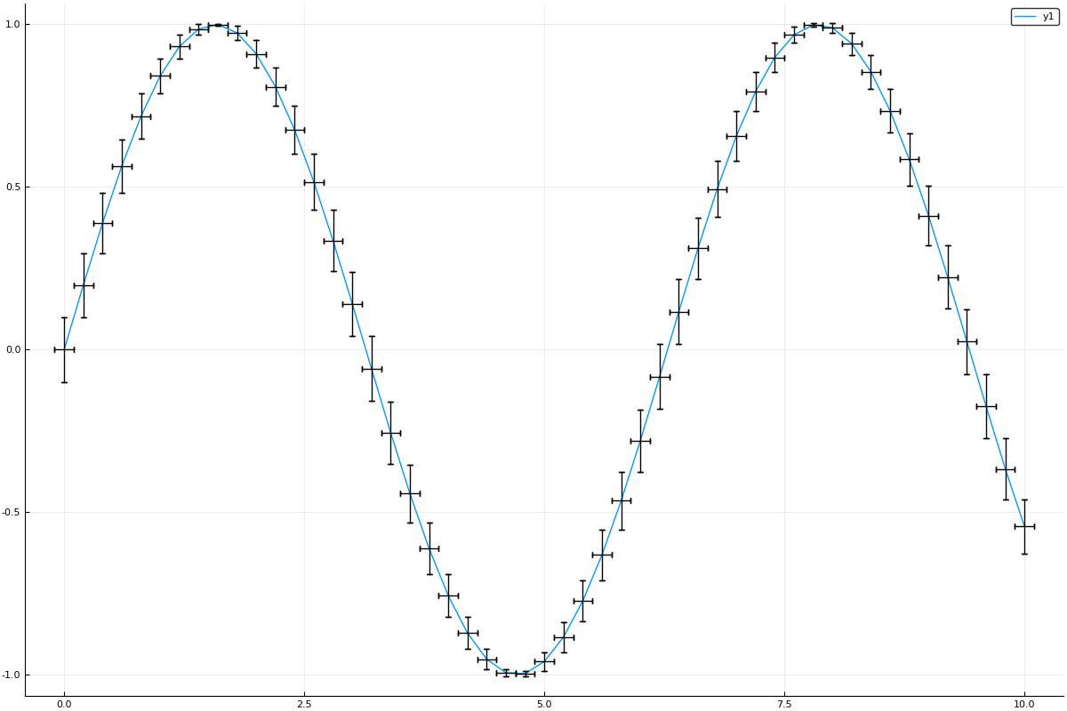

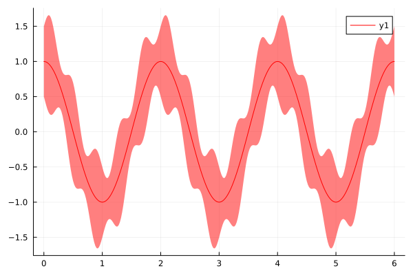
Displaying errors as a ribbon plot is also supported, but only for the y-axis uncertainty (a limitation inherited from Plots.jl due to how ribbon implements a fillrange).

julia> x = range(0, 6, 301)

julia> y = measurement.(cospi.(x), (5 .+ 2sinpi.(5x))/10)

julia> plot(x, y, uncertainty_plot = :ribbon, color = :red)