Charge Drift
Charged particles in vacuum move along the electric field lines under Coulomb's force, $\vec{F} = q \vec{E}$, where $\vec{F}$ corresponds to the force experienced by the particle, $q$ is the charge of the particle and $\vec{E}$ is the electric field. Charged particles in vacuum would be continuously accelerated until approaching the speed of light (called ballistic transport). However, inside a material, scattering prevents this constant acceleration and leads to a constant drift velocity
\[v_{d} = \mu E,\]
where $v_{d}$ is the drift velocity, $\mu$ the mobility and $E$ the electric field strength.
The scattering with matter not only limits the absolute drift velocity, it might also deviate the trajectories from the electric field lines: e.g., in crystals, the principal axes orientation has an impact on the resulting drift trajectory. The influence of the scattering on the drift trajectories can be expressed by a 3x3 tensor, the so-called mobility tensor $\mu_{ij}$, which transforms the electric field, $E$, into the drift velocity, $v_{i}$:
\[v_{i} = \mu_{ij} \cdot E_{j}.\]
The mobility varies for different materials and depends also on other parameters such as temperature, impurity density and the electric field strength, as explained later.
Charge Drift Models
Electrons and holes have different mobilities, resulting in different drift velocities. There are several models for the mobility tensor of electrons and holes in certain materials. Right now, two models are implemented. The first one is a pseudo-drift model, the ElectricFieldChargeDriftModel, which just takes the electric field vectors as drift vectors, see section Electric Field Charge Drift Model. The second one, ADLChargeDriftModel, is a drift model for high purity germanium, see section ADL Charge Drift Model. However, the implementation of an own model is possible and explained in section Custom Charge Drift Model.
Electric Field Charge Drift Model
The ElectricFieldChargeDriftModel describes a system in which electrons and holes move along the electric field lines. In this case, the mobility is a scalar $\pm$ 1 m²/(Vs) ($+$ for holes, and $-$ for electrons), and thus, the velocity field has the same (or opposite) direction as the electric field. Even though this model does not describe reality, it is useful in some cases to use the electric field vectors as velocity vectors.
In order to set the ElectricFieldChargeDriftModel for the simulation, the precision type of the calculation T (Float32 or Float64) has to be given as an argument. Note that T has to be of the same precision type of the simulation:
T = SolidStateDetectors.get_precision_type(sim) # e.g. Float32
charge_drift_model = ElectricFieldChargeDriftModel(T=T)
sim.detector = SolidStateDetector(sim.detector, charge_drift_model)
If no charge drift model is specified for the semiconductor of the detector in the configuration files, the default is ElectricFieldChargeDriftModel.
ADL Charge Drift Model
In high-purity germanium, the mobility cannot be expressed by a simple scalar quantity. Germanium has a cubic diamond lattice structure with $\langle$100$\rangle$, $\langle$110$\rangle$ and $\langle$111$\rangle$ as principal directions. Along these axes, the charge drift is parallel to the electric field. However, the longitudinal drift velocity, $v_{l}$, is not equally fast on the three axes.
On each axes, $v_{l}$ can be described through the parametrization proposed by D.M. Caughey and R.E. Thomas, which was later expanded by L. Mihailescu et al.:
\[v_l = \frac{\mu_0 E}{(1 + (E/E_0 )^{\beta})^{1/ \beta}} - \mu_{n} E.\]
The parameters $\mu_{0}$, $E_{0}$ and $\beta$ differ for electrons and holes, and $\mu_{n}$ is only relevant for electrons. These parameters were obtained by B. Bruyneel et al. in 2006 and by B. Bruyneel et al. in 2016 by measuring the drift velocities of electrons and holes in the $\langle$100$\rangle$ and $\langle$111$\rangle$ directions in high purity germanium at a temperature of 77 K. These parameters are stored in a configuration file, "drift_velocity_config.yaml" and "drift_velocity_config_2016.yaml" respectively, located in <package_directory>/examples/example_config_files/ADLChargeDriftModel. The configuration file is expressed as following:
model: ADLChargeDriftModel
phi110: -45°
material: HPGe
drift:
  velocity:
    model: Bruyneel2006
    parameters:
      e100:
        mu0: 38609cm^2/(V*s)
        beta: 0.805
        E0: 511V/cm
        mun: -171cm^2/(V*s)
      e111:
        mu0: 38536cm^2/(V*s)
        beta: 0.641
        E0: 538V/cm
        mun: 510cm^2/(V*s)
      h100:
        mu0: 61824cm^2/(V*s)
        beta: 0.942
        E0: 185V/cm
      h111:
        mu0: 61215cm^2/(V*s)
        beta: 0.662
        E0: 182V/cm
where the parameters are stored under the keys e100, e111, h100 and h111, in which e and h stand for electrons and holes, respectively, and 100 and 111, for the principal axes $\langle$100$\rangle$ and $\langle$111$\rangle$. In the 2016 publication, no e111 is given, instead the electron inter valley scattering rate is given. With these parameters the drift velocity can be calculated for the other axes.
model: ADL2016ChargeDriftModel
phi110: -45°
material: HPGe
drift:
  velocity:
    model: Bruyneel2016
    parameters:
      e100:
        mu0: 37165cm^2/(V*s)
        beta: 0.804
        E0: 507.7V/cm
        mun: -145cm^2/(V*s)
      escattering:
        eta0: 0.496
        b: 0.0296
        Eref: 1200V/cm
      h100:
        mu0: 62934cm^2/(V*s)
        beta: 0.735
        E0: 181.9V/cm
      h111:
        mu0: 62383cm^2/(V*s)
        beta: 0.749
        E0: 143.9V/cm
By default, in SolidStateDetectors.jl the $\langle$001$\rangle$ axis is aligned with the Z-axis of the coordinate system of the simulation. The crystal orientation can be set through the phi110 parameter, where the $\langle$001$\rangle$ axis is still aligned with the Z-axis and the angle between the $\langle$110$\rangle$ principal direction of the crystal and the X-axis is given by phi110. Alternatively, the crystal orientation can be set by passing a rotation matrix that describes the rotation from the global coordinate system to the crystal orientation system.
If the electric field is not aligned with any of the crystal axes, the charge drift velocity is not necessarily aligned with the electric field. In the ADLChargeDriftModel, two models are implemented to describe the charge drift of electrons and holes between the axes. Detailed information about the charge drift models is provided in the papers from L. Mihailescu et al. for electrons and from B.Bruyneel et al. for holes. Find the detailed calculations and modifications from the publications as implemented in SolidStateDetectors.jl here.
In order to perform the calculation of the drift velocities, a configuration file containing the parametrization values like the "drift_velocity_config.yaml" (with Bruyneel's data or modified values), has to be passed as an argument to the ADLChargeDriftModel or ADL2016ChargeDriftModel function. The precision of the calculation T (Float32 or Float64) has to be given as a keyword T. Note that T has to be of the same type as the chosen in the simulation:
T = SolidStateDetectors.get_precision_type(sim) # e.g. Float32
charge_drift_model = ADL2016ChargeDriftModel("<path_to_ADL_configuration_file>", T=T)
sim.detector = SolidStateDetector(sim.detector, charge_drift_model)
Default constructors such as ADL2016ChargeDriftModel() and ADL2016ChargeDriftModel(T=T) are also available. These automatically load the parameters from the files in <package_directory>/examples/example_config_files/ADLChargeDriftModel
The ADLChargeDriftModel can also be specified already in the configuration file as field charge_drift_model of the semiconductor of a detector, e.g.
detectors:
  semiconductor:
    # ...
    charge_drift_model:
        include: ADLChargeDriftModel/drift_velocity_config_2016.yaml
or
detectors:
  semiconductor:
    # ...
    charge_drift_model:
      model: ADLChargeDriftModel
      phi110: -0.785398 # in radians if no units are given
      material: HPGe
      drift: # ...
or
detectors:
  semiconductor:
    # ...
    charge_drift_model:
      model: ADLChargeDriftModel
      crystal_orientation:
        X: 45° # crystal axes correspond to the global xyz coordinate system, rotated 45° around the x axis
      material: HPGe
      drift: # ...
The charge_drift_model needs:
model: the name of the charge drift model, which in this case isADLChargeDriftModelphi110orcrystal_orientation: the description of the orientation of the crystal with respect to the global coordinate system. When usingphi110, the $\langle$001$\rangle$ axis is aligned with the globalzaxis andphi110describes the angle between the $\langle$110$\rangle$ axis and thexaxis in radians (counterclockwise, looking from the top). If the $\langle$001$\rangle$ axis is not aligned with thezaxis, a rotation matrix to transform the global coordinate system to the crystal axes system can be given.material(optional): the semiconductor material. If no material is given, thematerialof the semiconductor is taken by default.drift: the parameters needed to describe the longitudinal drift velocity along the $\langle$100$\rangle$ and $\langle$111$\rangle$ axes, see above.
The values from the default configuration file correspond to germanium at 77 K. Calculations of the drift velocities at other temperatures are also supported by the ADLChargeDriftModel. A parametrization for the temperature dependence of drift velocity, as a function of the electric field strength, $E$, was proposed by M.A. Omar and L. Reggiani:
\[\quad\mu_0(T) = A/T^P~, \quad V_s(T) = B\tanh^{1/2}(\theta/2T) \]
Note that the saturation velocity, $V_s$, is related to $E_0$ via
\[E_0(T) = V_s(T)/\mu_0(T)\]
The four parameters, $A$, $P$, $B$, $\theta$, are different for electrons and holes. This model can be used to scale the $\mu_{0}$ and $E_{0}$ parameters of the ADLChargeDriftModel directly as follows:
\[\mu_0(T) = \mu_0(77K) \left(\frac{T}{77K}\right)^{-P}~, \quad E_0(T) = E_0(77K) \sqrt{\frac{\tanh(\theta/2T)}{\tanh(\theta/2 \cdot 77K)}} \frac{\mu_0(77K)}{\mu_0(T)}\]
The implementation of the model can be found in the directory <package_directory>/src/ChargeDriftModels/ADLChargeDriftModel/TemperatureModels. To use this in the calculation of the drift velocities, the corresponding configuration file, the temperature and the precision must be given to the function.
T = SolidStateDetectors.get_precision_type(sim) # e.g. Float32
charge_drift_model = ADL2016ChargeDriftModel("<path_to_ADL_configuration_file>", T = T, temperature = 100u"K")
sim.detector = SolidStateDetector(sim.detector, charge_drift_model)
If no temperature is given as a parameter, the calculations will be performed at a default temperature of 77 K. If no configuration file is given, the default config file <package_directory>/examples/example_config_files/ADLChargeDriftModel/drift_velocity_config_2016.yaml is loaded. In charge drift configuration files, the M.A. Omar and L. Reggiani parametrization can be used by adding the following temperature_dependence field like this:
temperature_dependence:
  reference_temperature: 77K
  model: Omar1987
  parameters:
    e:
      p: 1.68
      theta: 200K
    h:
      p: 2.4
      theta: 200K
For convenience, this model can already be found in the drift_velocity_config.yaml and drift_velocity_config_2016.yaml example config files.
The default parameters used in this model were calculated by M.A. Omar and L. Reggiani before the publication of the ADLChargeDriftModel parameters, with $\beta = 2$. Thus, the use of this model to scale the drift parameters in ADLChargeDriftModel or ADL2016ChargeDriftModel is considered experimental.
Inactive Layer Charge Drift Model
The InactiveLayerChargeDriftModel describes a system in which electrons and holes move along the electric field lines. The mobilities for electrons and holes are scalar ($+$ for holes, and $-$ for electrons), and thus, the velocity field has the same (or opposite) direction as the electric field.
The mobilities are calculated considering three major scattering processes: scattering off ionized impurities, neutral impurities and acoustic phonons. Thus, the mobilities depend on the impurity concentrations and temperature.
The precision of the calculation T (Float32 or Float64) has to be given as a keyword T. Note that T has to be of the same type as the chosen in the simulation:
The InactiveLayerChargeDriftModel can be specified in the configuration file as field charge_drift_model of the semiconductor of a detector, e.g.
detectors:
  semiconductor:
    temperature: 90K  # temperature must be defined here for InactiveLayerChargeDriftModel
    # ...
    charge_drift_model:
      model: InactiveLayerChargeDriftModel
      # temperature: 90K  # optional: if provided, must match semiconductor.temperature (used for validation only)
      bulk_impurity_density:
        name: constant
        value: -1e10cm^-3
      surface_impurity_density:
        name: li_diffusion
        lithium_annealing_temperature: 623K
        lithium_annealing_time: 18minute
        doped_contact_id: 2
      neutral_impurity_density:
        name: constant
        value: 5.6769e15cm^-3
The charge_drift_model needs:
model: the name of the charge drift model, which in this case isInactiveLayerChargeDriftModel.temperature(optional): if provided, validated againstsemiconductor.temperature— both must match or an error is raised. Temperature must be defined in thesemiconductorand cannot be set only inside the charge drift model, because it is also used independently for diffusion calculations during charge drift.bulk_impurity_density(optional): the density of the p-type impurity in the crystal.surface_impurity_density(optional): the density profile of lithium (n-type) in the surface layer.neutral_impurity_density: the density profile of the non-ionized impurity in the crystal.
The fields bulk_impurity_density and surface_impurity_density do not need to be explicitly defined if PtypePNJunctionImpurityDensity is chosen as the overall impurity density profile.
The temperature must be defined in semiconductor.temperature — it cannot be set only inside the charge drift model config, because the semiconductor temperature is also used independently for diffusion calculations during charge drift. Optionally, a temperature field can be added to the charge_drift_model config for validation: if provided, it must match semiconductor.temperature or an error is raised. If semiconductor.temperature is not set, a material-specific default is used (77 K for High Purity Germanium, 293 K otherwise) and a warning is issued — this applies even if a temperature is specified in the charge drift model config, since that field only validates, not sets, the semiconductor temperature.
Custom Charge Drift Model
The user can implement and use their own drift model.
The first step is to define a struct for the model which is a subtype of SolidStateDetectors.AbstractChargeDriftModel:
using SolidStateDetectors
using SolidStateDetectors: SSDFloat, AbstractChargeDriftModel

struct CustomChargeDriftModel{T <: SSDFloat} <: AbstractChargeDriftModel{T}
    # optional fields to parameterize the model
end
The second step is to define two methods (getVe for electrons and getVh for holes), which perform the transformation of an electric field vector, fv::SVector{3,T}, into a velocity vector. Note, that the vectors are in cartesian coordinates, independent of the coordinate system (cartesian or cylindrical) of the simulation. Even if not used, the third argument of getVe and getVh should be a CartesianPoint{T}, which also allows defining position-dependent mobility models.
using StaticArrays
function SolidStateDetectors.getVe(fv::SVector{3, T}, cdm::CustomChargeDriftModel, current_pos::CartesianPoint{T})::SVector{3, T} where {T <: SSDFloat}
    # arbitrary transformation of fv, optionally position dependent
    return -fv
end

function SolidStateDetectors.getVh(fv::SVector{3, T}, cdm::CustomChargeDriftModel, current_pos::CartesianPoint{T})::SVector{3, T} where {T <: SSDFloat}
    # arbitrary transformation of fv, optionally position dependent
    return fv
end
Then, one can apply the model to the simulation:
T = SolidStateDetectors.get_precision_type(sim) # e.g. Float32
charge_drift_model = CustomChargeDriftModel{T}()
sim.detector = SolidStateDetector(sim.detector, charge_drift_model)
Charge Trapping Models
Electrons and holes can be trapped on their way to the contacts, resulting in a decrease in height of the observed charge pulse. SolidStateDetectors.jl allows for incorporating and testing different charge trapping models.
In order to implement a charge trapping model, the first step is to define a struct for the model which is a subtype of SolidStateDetectors.AbstractChargeTrappingModel:
using SolidStateDetectors
using SolidStateDetectors: SSDFloat, AbstractChargeTrappingModel

struct CustomChargeTrappingModel{T <: SSDFloat} <: AbstractChargeTrappingModel{T}
    # optional fields to parameterize the model
end
The second step would be to define a method for _calculate_signal, which returns a charge signal based on a given charge drift path and its pathtimestamps, the charge value of the charge cloud, the interpolated weighting potential wpot and the point_types to infer the coordinate system type S (Cartesian or Cylindrical):
using SolidStateDetectors: SSDFloat
using Interpolations
function SolidStateDetectors._calculate_signal(
        ctm::CustomChargeTrappingModel{T},
        path::AbstractVector{CartesianPoint{T}},
        pathtimestamps::AbstractVector{T},
        charge::T,
        wpot::Interpolations.Extrapolation{T, 3},
        point_types::PointTypes{T, N, S}
    )::Vector{T} where {T <: SSDFloat, N, S}

    # Implement method here
endSo far, the charge trapping models do not influence the charge drift path simulation, but just the signal calculation afterwards.
NoChargeTrappingModel
If no charge trapping model is selected, the default is the NoChargeTrappingModel. In this case, the signal is calculated using the Shockley-Ramo theorem, i.e. by evaluating the weighting potential wpot at every point path[i] of the charge drift path and multiplying it with the charge of the charge cloud.
BoggsChargeTrappingModel
In SolidStateDetectors.jl, the Boggs charge trapping model implemented is the one presented in Boggs et al. (2023). In this model, the charge cloud loses part of its charge at every point path[i] of the charge drift, depending on its drift and thermal velocity, as well as the trapping product $[n\sigma_{e/h}]^{-1}$ for electrons and holes. The charge signal is then given by the charge-decreased charge cloud reaching the contacts and the charges trapped on the way.
The BoggsChargeTrappingModel can be applied in the configuration file by adding a field charge_trapping_model to the semiconductor with model: Boggs and parameters defining the (inverse) trapping products and (optionally) the temperature:
detectors:
  - semiconductor:
      material: #...
      temperature: 78K  # preferred: define temperature here
      geometry: #...
      charge_trapping_model:
        model: Boggs
        parameters:
          nσe-1: 1020cm
          nσh-1: 2040cm
          # temperature: 78K  # optional: if provided, must match semiconductor.temperature

# ... or ...

detectors:
  - semiconductor:
      material: #...
      temperature: 78K  # preferred: define temperature here
      geometry: #...
      charge_trapping_model:
        model: Boggs
        parameters:
          nσe: 0.001cm^-1
          nσh: 0.0005cm^-1
# temperature: 78K # optional: if provided, must match semiconductor.temperatureThe temperature is preferably defined in semiconductor.temperature and will be passed automatically to the trapping model. A temperature field can also be specified inside parameters; if both are provided they must match or an error is raised. Unlike the charge drift model, if no semiconductor.temperature is defined, a temperature inside parameters alone is also accepted. If semiconductor.temperature is not set, a material-specific default is used (77 K for High Purity Germanium, 293 K otherwise) and a warning is issued — this applies even if a temperature is specified inside parameters, since the semiconductor temperature is always resolved first and passed to the trapping model.
It can also be applied to an already read-in SolidStateDetector using for example:
using SolidStateDetectors, Unitful
T = Float32
sim = Simulation{T}(SSD_examples[:InvertedCoax])

parameters = Dict("parameters" =>
  Dict("nσe-1" => 1000u"cm", "nσh-1" => 500u"cm", "temperature" => 78u"K"))
sim.detector = SolidStateDetector(sim.detector, BoggsChargeTrappingModel{T}(parameters))
ConstantLifetimeChargeTrappingModel
This constant-lifetime-based charge trapping model assumes electrons and holes to have a constant free lifetime throughout the crystal. In this model, the charge cloud loses part of its charge at every point path[i] of the charge drift, depending on the lifetime. The charge signal is then given by the charge-decreased charge cloud reaching the contacts and the charges trapped on the way.
This idea is presented in Dai et al. (2023).
Besides, the model implemented has two sets of parameters for the sensitive (bulk) and inactive (dead layer/surface layer) volume respectively.
The ConstantLifetimeChargeTrappingModel can be applied in the configuration file by adding a field charge_trapping_model to the semiconductor with model: ConstantLifetime and parameters defining the constant lifetime:
detectors:
  - semiconductor:
      material: #...
      geometry: #...
      charge_trapping_model:
        model: ConstantLifetime
        parameters:
          τh: 1ms
          τe: 1ms
The ConstantLifetimeChargeTrappingModel can also be applied to an already read-in SolidStateDetector, for example:
using SolidStateDetectors, Unitful
T = Float64
sim = Simulation{T}(SSD_examples[:TrueCoaxial])
simulate!(sim)

# only model the sensitive volume
τh = τe = 1u"ms"
parameters = Dict("parameters" => Dict("τh" => τh, "τe" => τe))

# pass the trapping model to the `sim.detector`
sim.detector = SolidStateDetector(sim.detector, ConstantLifetimeChargeTrappingModel{T}(parameters))
CombinedChargeTrappingModel
The CombinedChargeTrappingModel allow to run a charge trapping model inside the bulk and a different charge trapping model inside the inactive layer using model_inactive and parameters_inactive entries in the yaml file. If model_inactive is present in the yaml file but equals to nothing, NoChargeTrappingModel will be used by default in the inactive layer. Combinations supported by this model:
- Bulk: Boggs CTM, inactive layer: Constant lifetime CTM
charge_trapping_model:
      model: Boggs
      parameters:
        nσe-1: 1020cm
        nσh-1: 2040cm
      model_inactive: ConstantLifetime
      parameters_inactive:
        τh: 1μs
τe: 1μs- Bulk: Constant lifetime CTM, inactive layer: Constant lifetime CTM
charge_trapping_model:
      model: ConstantLifetime
      parameters:
        τh: 1ms
        τe: 1ms
      model_inactive: ConstantLifetime
      parameters_inactive:
        τh: 1μs
        τe: 1μs
This model also allows disabling the charge trapping model inside the inactive layer by having model_inactive: and the bulk by deleting model: from the charge_trapping_model: block. If inactive_layer_geometry is passed to the yaml file, this is the region used for the inactive layer charge trapping model, else, the model will use the inactive layer geometry defined by the impurity density model (PtypePNJunctionImpurityDensity) using the point types.
The temperature is preferably defined in semiconductor.temperature and will be passed automatically. Optionally, a temperature field can be added at the top level of the charge_trapping_model config (i.e. alongside model and model_inactive, not inside parameters); if both are provided they must match or an error is raised. Unlike the charge drift model, if no semiconductor.temperature is defined, a top-level temperature in the charge_trapping_model alone is also accepted. If semiconductor.temperature is not set, a material-specific default is used (77 K for High Purity Germanium, 293 K otherwise) and a warning is issued — this applies even if a temperature is specified in the charge_trapping_model config, since the semiconductor temperature is always resolved first and passed to the trapping model.
using SolidStateDetectors, Unitful
T = Float64
sim = Simulation{T}(SSD_examples[:TrueCoaxial])
simulate!(sim)

# model both the sensitive and inactive volumes based on a user-defined `inactive_layer_geometry`
τ, τ_inactive = 1u"ms", 100u"ns"
## define the inactive_layer_geometry, an example:
inactive_layer_geometry_dict = Dict(
        "tube" => Dict(
            "r" => Dict("from" => 1.0u"mm", "to" => 10.0u"mm"),
            "h" => 5.0u"mm",
            "origin" => Dict("z" => 2.5u"mm")
        )
    )
using SolidStateDetectors: AbstractGeometry, parse_CSG_transformation, combine_transformations, Geometry, construct_units
outer_transformations = parse_CSG_transformation(T, sim.config_dict["detectors"][1], sim.input_units)
inner_transformations = parse_CSG_transformation(T,sim.config_dict["detectors"][1]["semiconductor"], sim.input_units)
transformations = combine_transformations(inner_transformations, outer_transformations)
inactive_layer_geometry = Geometry(T, inactive_layer_geometry_dict, sim.input_units, transformations)
## or simply use the already constructed geometry if the `inactive_layer_geometry ` geometry is defined in the configuration file
# inactive_layer_geometry = sim.detector.semiconductor.charge_trapping_model.inactive_layer_geometry

parameters = Dict("model" => "ConstantLifetime", "model_inactive" => "ConstantLifetime", "parameters" => Dict("τh" => τ, "τe" => τ), "parameters_inactive" => Dict("τh" => τ_inactive, "τe" => τ_inactive), "inactive_layer_geometry" => inactive_layer_geometry)
# pass the trapping model to the `sim.detector`
sim.detector = SolidStateDetector(sim.detector, CombinedChargeTrappingModel{T}(parameters))
Group Effects
The movement of electrons and holes is not only given by the forces resulting from external electric fields. In addition, diffusion and self-repulsion of the charge carriers can play a significant role when simulating drift paths. To simulate this, electron and holes cannot be described as single point-like charges anymore, but as charge clouds consisting of multiple point-like charges. SolidStateDetectors.jl offers different models for the Initial Charge Cloud Distribution. Right now, Diffusion and Self-Repulsion are implemented as experimental features.
Initial Charge Cloud Distribution
Electron and hole clouds can be easily constructed using NBodyChargeCloud. An NBodyChargeCloud consists of a center point charge, surrounded by shells of equally distributed point charges. SolidStateDetectors.jl provides two constructors for an NBodyChargeCloud, depending on how the charges in the shells should be distributed. For charge clouds consisting of few charges (less than around 50), the shells should consist of Platonic Solids, whereas for higher numbers of charges, the points in the shells should be Equally Distributed on a Regular Sphere.
Platonic Solids
One way of defining an NBodyChargeCloud is having a center point charge surrounded by shells with point charges on the vertices of platonic solids. For now, all shells will have the same number of charges and be oriented the same way.
center = CartesianPoint{T}(0,0,0)
energy = 1460u"keV"
nbcc = NBodyChargeCloud(center, energy)
plot(nbcc)
Equally Distributed on a Regular Sphere
For an NBodyChargeCloud consisting of more than around 50 charges, the shells should consist of more than 20 point charges and the approach with using Platonic Solids for the shell structure might not be favored anymore. For this, a second algorithm was implemented that generates point charges equally distributed on the surface of a regular sphere. The approximate number of charges needs to be passed to the constructor of NBodyChargeCloud to use this method.
center = CartesianPoint{T}(0,0,0)
energy = 1460u"keV"
nbcc = NBodyChargeCloud(center, energy, 100)
plot(nbcc)
Diffusion
Diffusion describes the random thermal motion of charge carriers. In SolidStateDetectors.jl, diffusion is simulated using a random walk algorithm. Diffusion is simulated using fixed-step vectors where the magnitude of the step vectors depends on the diffusion constant $D$ and the time steps $\Delta t$.
center = CartesianPoint{T}(0,0,0)
energy = 1460u"keV"
nbcc = NBodyChargeCloud(center, energy, 100)
evt = Event(nbcc)
simulate!(evt, sim, diffusion = true, end_drift_when_no_field = true)
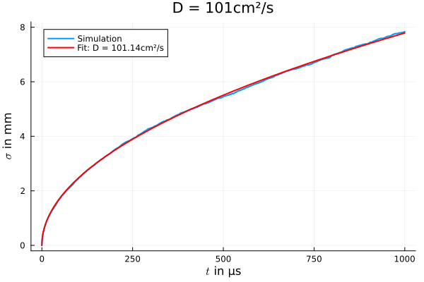
In the absence of an external electric field, the size (standard deviation $\sigma$) of the charge cloud is expected to evolve with $\sigma = \sqrt{6 D t}$ (in three dimensions), where $t$ is the time. Thus, the diffusion constant determines the time evolution of the charge cloud size.
For an initial charge cloud of 1000 point charges, all located at the origin of the coordinate system, and a diffusion constant of $101\,\text{cm}^2\text{/s}$, the random walk algorithm results in the expected $\sqrt{t}$ dependence. A fit of $\sigma = \sqrt{6Dt}$ shows that the diffusion constant with which the charge cloud evolves matches the input value for $D$.
The diffusion constants for electrons and holes are stored in SolidStateDetectors.material_properties as De and Dh, respectively. For high-purity germanium at $T=77\,\text{K}$, the diffusion constants for electrons and holes are reported to be $D_e = 239\,\text{cm}^2\text{/s}$ and $D_h = 279\,\text{cm}^2\text{/s}$. These values are the default values in SolidStateDetectors.material_properties:
SolidStateDetectors.material_properties[:HPGe]Electrons: 239 cm^2 s^-1
Holes: 279 cm^2 s^-1Values for De and Dh in SolidStateDetectors.material_properties can be given with or without units. If no units are passed, the values are interpreted as having the unit m$^2$/s.
Self-Repulsion
After the creation of electron-hole pairs, both the electron and the hole clouds repel each other. The electric field of a point-charge, $q$, at a distance to the charge, $\vec{r}$, is given by
\[\vec{E} = \frac{1}{4\pi\epsilon_0\epsilon_r} \frac{q}{r^2} \vec{e}_r\]
SolidStateDetectors.jl does not account for attraction of electrons and holes but only for repulsion of charge carriers of the same type. The determination of the electric field vector is calculated pair-wise for each pair of charge carriers.
center = CartesianPoint{T}(0,0,0)
energy = 1460u"keV"
nbcc = NBodyChargeCloud(center, energy, 100)
evt = Event(nbcc)
simulate!(evt, sim, self_repulsion = true, end_drift_when_no_field = true)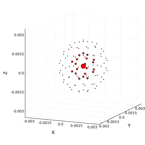
Combination of Group Effects
Diffusion and Self-Repulsion can be simulated both at once to get the most realistic picture:
center = CartesianPoint{T}(0,0,0)
energy = 1460u"keV"
nbcc = NBodyChargeCloud(center, energy, 100)
evt = Event(nbcc)
simulate!(evt, sim, diffusion = true, self_repulsion = true, end_drift_when_no_field = true)
However, be aware that simulations including group effects will result in significantly longer simulation times.