A digital optics laboratory

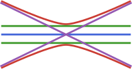
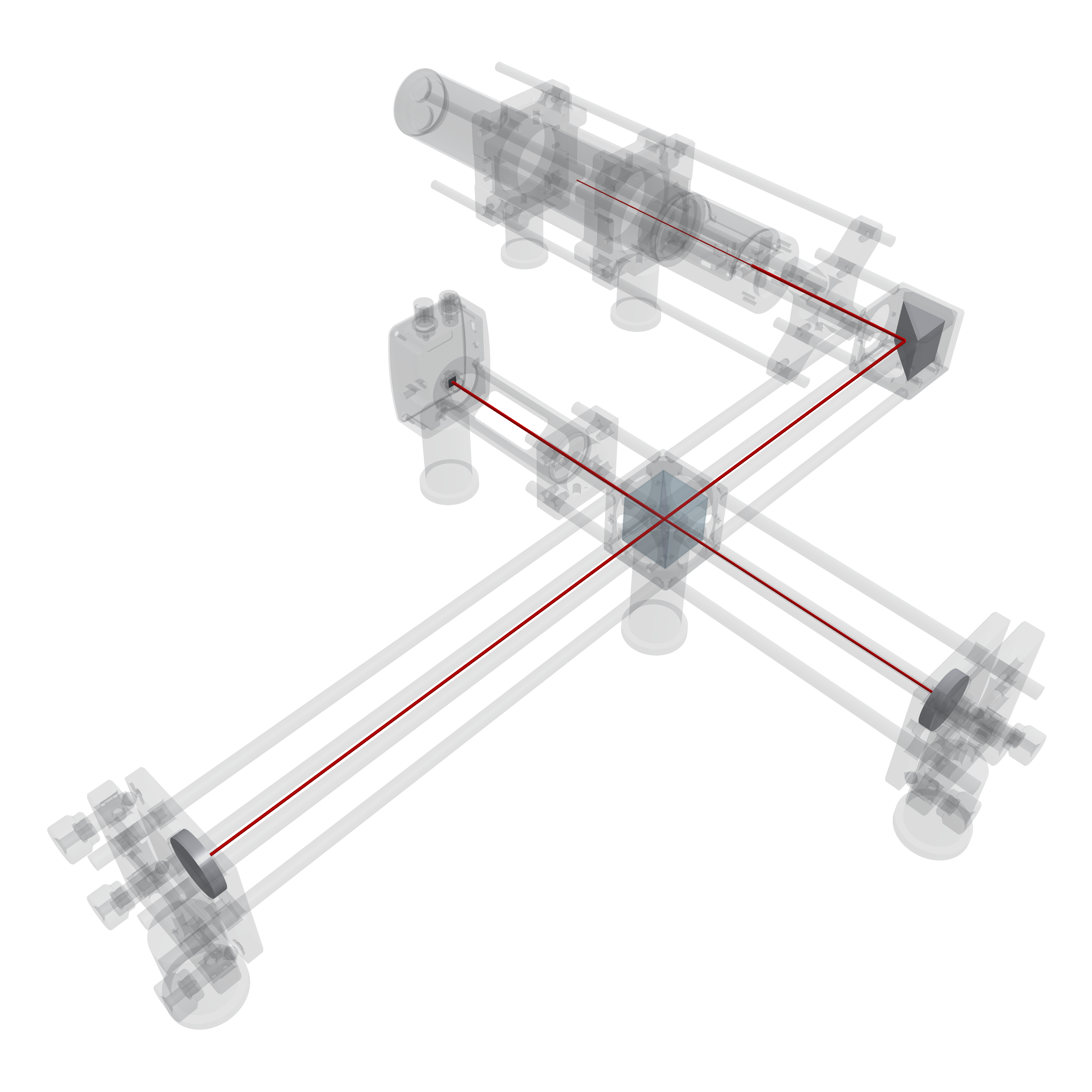
Building optical setups in a laboratory environment – for instance a laser interferometer – is a common task for optical engineers and physicists. This package is intended to provide a simulation environment in which the user can quickly analyze and layout simple optical components like lenses or beamsplitters before committing to a breadboard setup.

What is the purpose of this package ​

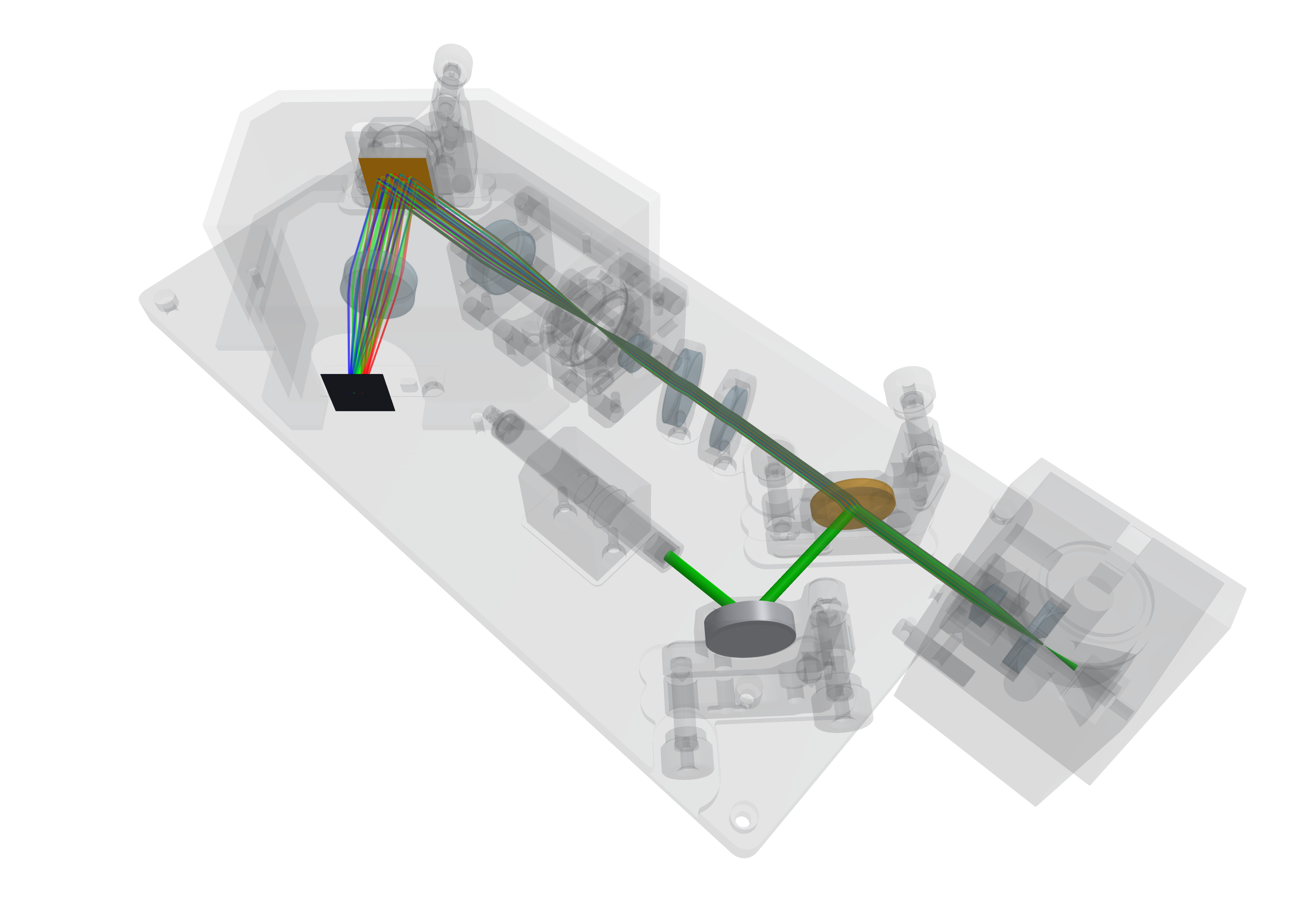
This package mainly tries to provide a simple Gaussian beamlet propagation tool for coherent, monochromatic and directed light sources. It also offers a convenient kinematic API that allows for the easy placing of optical elements and straight-forward simulation of moving or vibrating components.

For this purpose, the package implements a traditional ray tracing solver. This forms the backbone of the Gaussian beamlet tracing scheme that has been implemented to model the propagation of laser beams.

BMO in 30 seconds ​

A circularly polarized Gaussian laser beam through a Keplerian beam expander – beam radius, focus and polarization are traced along with the rays.

using GLMakie, BeamletOptics

const mm = 1e-3

# Keplerian beam expander: f₁ = 15 mm, f₂ = 45 mm → 3× magnification
lens1 = ThinLens(15mm, 15mm, 12mm, 1.5)      # biconvex, f = R for n = 1.5
lens2 = ThinLens(45mm, 45mm, 25mm, 1.5)
translate3d!(lens1, [0, 20mm, 0])
translate3d!(lens2, [0, 80mm, 0])              # spacing f₁ + f₂
system = System([lens1, lens2])

# 532 nm laser, 1.5 mm waist radius, circularly polarized
laser = AstigmaticGaussianBeamlet([0, 0, 0], [0, 1, 0], 532e-9, 1.5mm; E0=[1, 0, im]/√2)
solve_system!(system, laser)

# plot lenses and beam
fig = Figure(size=(800, 300))
ax = LScene(fig[1, 1], show_axis=false)
render!(ax, system)
render!(ax, laser; color=RGBAf(0.1, 0.8, 0.1, 0.25), flen=0.04,
        show_polarization=true, pol_λ=4mm, pol_gain_max=4, pol_scale=1.5)
render_lcs!(ax, [-5mm, 50mm, -25mm]; scale=3, show_labels=true)
set_orthographic(ax)

  0.0         0.0         0.0           1.0             # hide

# beam radius behind the expander relative to the input beam
gauss_parameters(laser, 0.12)[1] / gauss_parameters(laser, 0.0)[1]

2.9493488872847196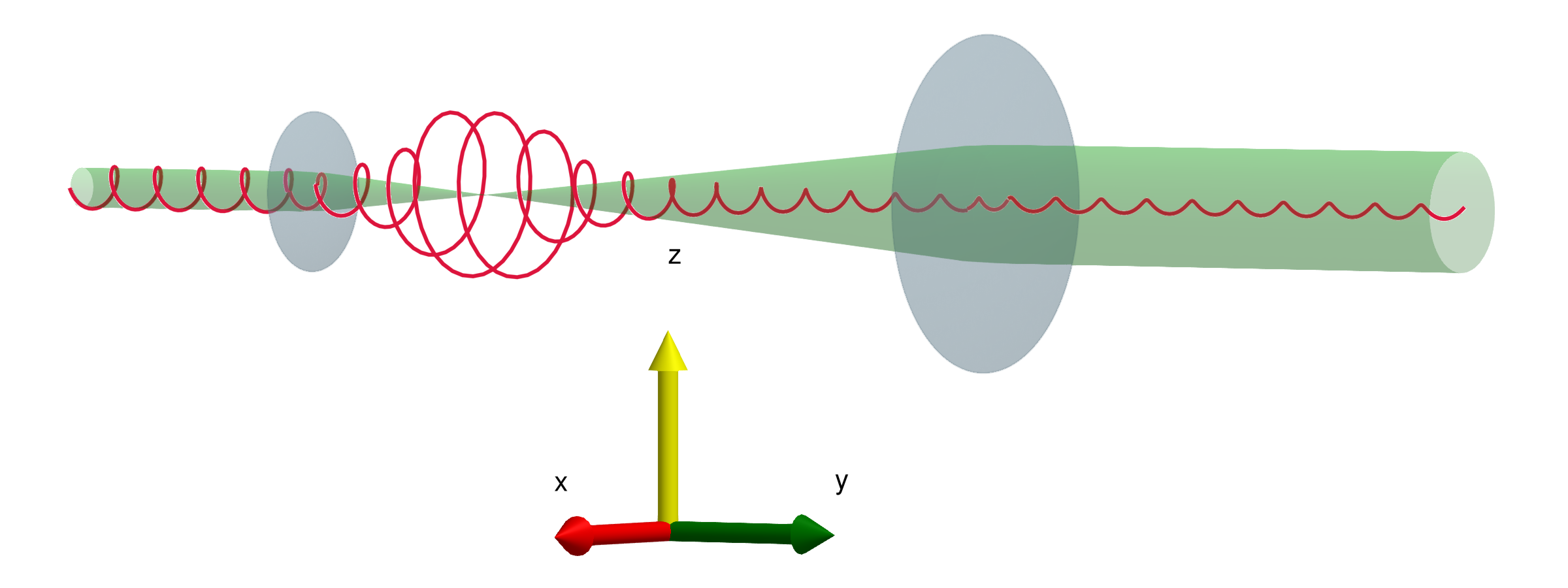

Resources to get you started ​

Browse all tutorials and examples

Installation ​

You can add this package to your project by entering the package manager (press ] in the REPL) and typing add BeamletOptics. It is also recommended that you add GLMakie. You can include this package into your current scope via using BeamletOptics. If a Makie version is loaded before or after the inclusion of this package, the extension provided as part of this package will enable additional visualization functions.

Citation and license ​

The BeamletOptics package is made available under the MIT license. If you use this package for your research, we encourage you to cite it. For your convenience, a BibTeX entry is provided as part of the package (CITATION.bib) or on Zenodo.

Similar packages ​

A variety of packages and tools exist that implement similar approaches or offer optics modeling capabilities.

There also exists a plethora of commercial and non-commercial simulation frameworks outside of the Julia ecosystem. For specific examples regarding the beamlet method used in this package, refer to the Complex ray tracing section.