Point spread functions

A Detector placed in the focal plane of an imaging system yields an estimate of its point spread function (PSF), see the Point spread function estimation section for the general idea. The examples below cover the diffraction limited case, an aberrated system and the vectorial focus at high NA.

Collimated input

When dealing with a collimated source as the input to your optical system, where you want to calculate the PSF, DO NOT use the CollimatedSource beam group directly but instead use the UniformDiscSource constructor. This function returns a CollimatedSource with an equal-area sampling, which correctly weights the outer beams in relation to the inner beams. Otherwise the results might be wrong.

Airy disc

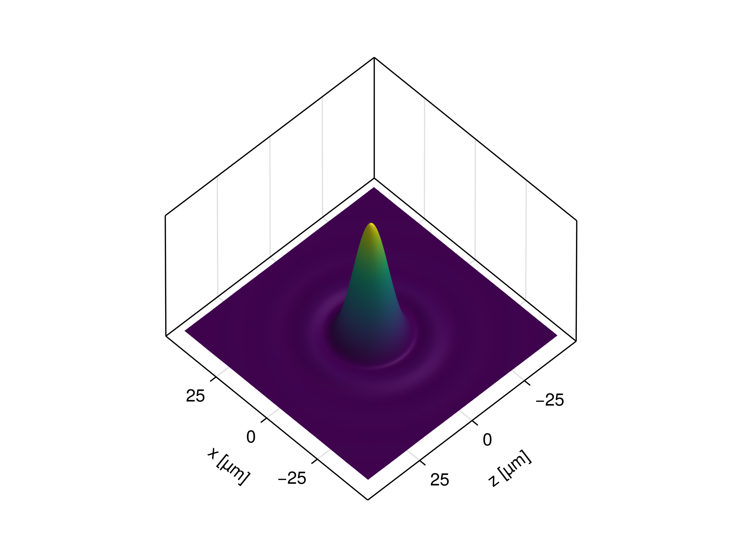
This is a classic example where a collimated circular beam is imaged onto a point by a singlet lens. Due to the finite size of the aperture stop (in this case given by the 15 mm size of the beam), the diffraction limited intensity pattern is given by the Airy-disc:

With the radius from the origin, the maximum intensity, the Bessel function of the first kind of order one, the aperture width, the wavelength and the focal length .

# example parameters
l = 1e-3
R1 = 100e-3
R2 = Inf
d = 25.4e-3
n = 1.5
λ = 1e-6

# generate uniform source, lens and detector
cs = UniformDiscSource([0, -10mm, 0], [0, 1, 0], 15e-3, λ)
lens = SphericalLens(R1, R2, l, d, x -> n)
detector = Detector(10e-3)

# shift detector into focus
translate3d!(detector, [0, 200mm + 0.13mm, 0])

# build system
sys = System([lens, detector])

solve_system!(sys, cs)

# retrieve intensity
x, z, I_num = intensity(detector; n=500, crop_factor=10)

Visualizing the result yields the expected Airy-disk pattern.

Coma and astigmatism

In this example, an aspheric lens images the collimated source onto a point but is tilted around the x-axis by 0.5 degrees. This results in aberrations distorting the stigmatic imaging and leading to coma and astigmatism.

k = -0.675
d = 75.0e-3
l = 15e-3
radius = 76.68e-3
A = [0*(1e3)^1, 2.7709219e-8*(1e3)^3, 6.418186e-13*(1e3)^5, -1.5724014e-17*(1e3)^7, -2.7768768e-21*(1e3)^9, -2.590162e-25*(1e3)^11]
AL75150 = Lens(
    EvenAsphericalSurface(radius, d, k, A),
    l,
    n -> 1.5006520430
)

xrotate3d!(AL75150, deg2rad(-0.5))

detector = Detector(15e-3)

translate3d!(detector, [0, 158.1779e-3, 0.0])
system = System([AL75150, detector])

ps = UniformDiscSource([0, -0.1, 0], [0,1,0], 0.8*d, 1550e-9)

solve_system!(system, ps)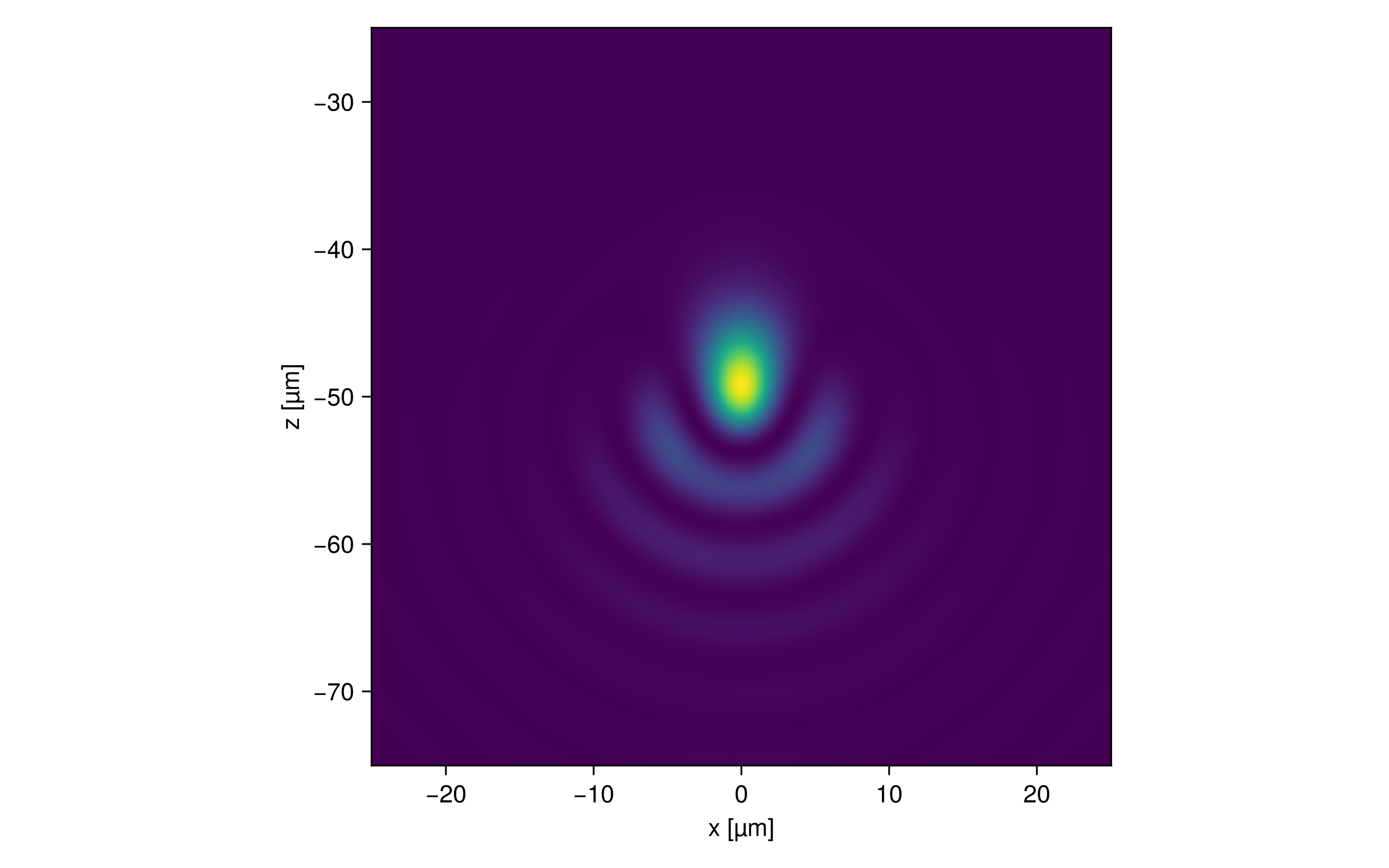

Vectorial focusing at high NA

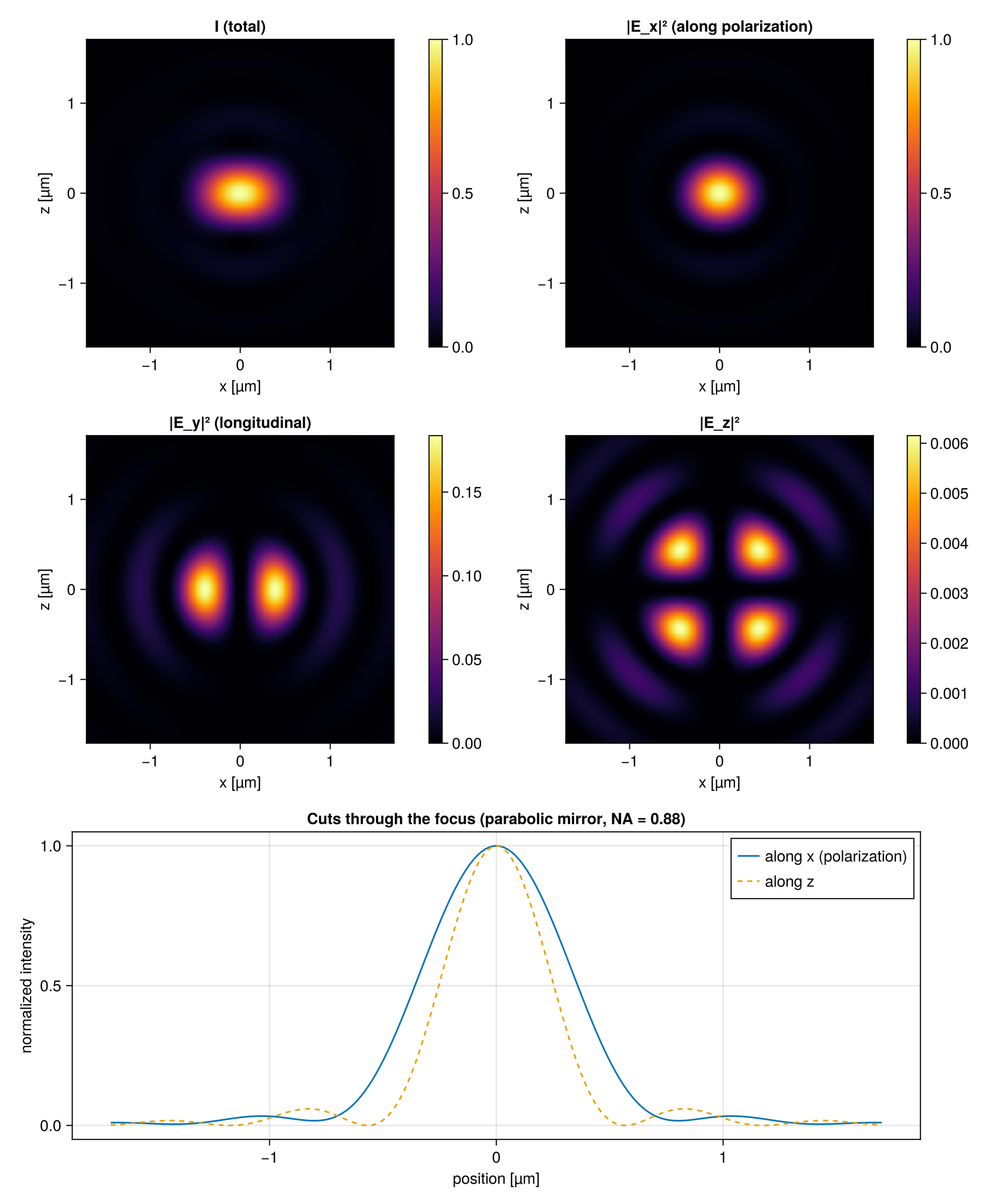
When a system is traced with PolarizedRays, the detector adds the field vectors E0 of all rays coherently as 3D vectors instead of scalar phasors. For small numerical apertures (NA) this reproduces the scalar result, since all field vectors are nearly parallel. At high NA, however, the rays converge from steep angles and their field vectors tilt towards the optical axis. As described by Richards and Wolf [4], this has two visible consequences for a linearly polarized input:

• the PSF is stretched along the direction of the input polarization, and

• a longitudinal field component (along the optical axis) appears, which vanishes on axis but forms two lobes along the polarization direction.

In this example an on-axis ParabolicMirror focuses a collimated, -polarized beam. A paraboloid images an on-axis point at infinity without aberrations for any aperture, so the resulting PSF is limited only by diffraction. With a focal length of 5 mm and a 12 mm beam the numerical aperture is   .

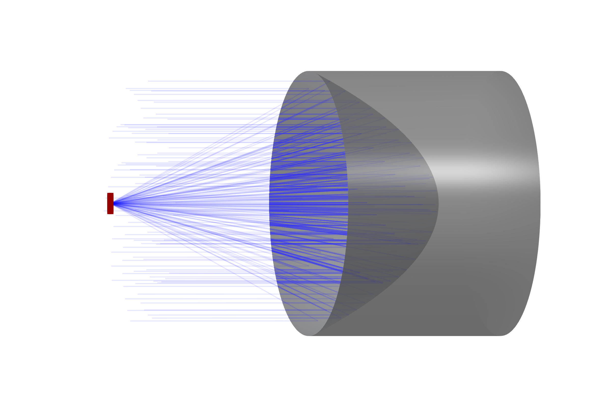
The mirror vertex lies at the origin and its focus at  . The detector is placed in the focal plane, so it sits in front of the mirror on the path of the incoming beam. To prevent the detector from clipping the incoming rays, the beam is spawned between the detector and the mirror rim.

Polarized collimated beam

UniformDiscSource spawns unpolarized Rays. The polarized source is built from its equal-area sampling by replacing each ray with a PolarizedRay of the same position and direction.

using BeamletOptics
const BMO = BeamletOptics

λ = 1e-6
f = 5e-3
D = 12e-3

mirror = ParabolicMirror(f, 12.5e-3)

# spawn the beam behind the detector (y = -f) and in front of the mirror rim (y ≈ -1.95 mm)
src = UniformDiscSource([0, -f / 2, 0], [0, 1, 0], D, λ; num_rays = 5000)
pol_src = CollimatedSource(
    [Beam(position(first(rays(b))), direction(first(rays(b))), λ, [1.0, 0, 0]) for b in BMO.beams(src)], D, [0, -f / 2, 0], [0, 1, 0])

pd = Detector(1e-3)
translate3d!(pd, [0, -f, 0])

solve_system!(System([mirror, pd]), pol_src)

NA = sin(2 * atan(D / (4f)))
R = 1.5λ / NA
xs, zs, E = electric_field(pd; n = 201, x_min = -R, x_max = R, z_min = -R, z_max = R)

I  = intensity.(E)                # total intensity
Ey = map(e -> abs2(e[2]), E)      # longitudinal component

The field E is a matrix of complex 3D vectors, so individual components can be evaluated separately. The cuts through the focus show a full width at half maximum of about 720 nm along and 510 nm along , i.e. the PSF is roughly 1.4 times wider along the polarization. The longitudinal component reaches about 18 % of the peak of the transverse component.

Ray amplitudes at high NA

The field vector E0 of a PolarizedRay carries the Fresnel/Jones amplitude coefficients, but neither the change of the ray-tube cross-section nor the refractive intensity factor . A real trace therefore weights the marginal rays differently than an energy-conserving (Debye) calculation. Geometry, phases and field directions are unaffected, but the PSF shape deviates quantitatively at high NA:

• ideal mirrors ( ) only lack the ray-tube factor; for an on-axis ParabolicMirror at NA 0.88 the normalized intensity cuts deviate by about 2 %,

• refractive surfaces additionally overweight rays exiting glass at steep angles ( ); for a hyperbolic singlet with   at NA 0.78 the FWHM ratio along/across the polarization becomes roughly 1.5 instead of 1.25.