Laser alignment

Before you start

This tutorial assumes basic familiarity with Julia. If you are new to the language, the Getting started section of the Julia manual and the Julia learning resources are good starting points; Modern Julia Workflows covers package environments and editor setup.

We also assume that you run the code in VS Code with the Julia extension installed. Execute the code blocks one after another in the integrated Julia REPL, e.g. by selecting them and pressing Shift+Enter. You need to install the packages once beforehand: press ] in the REPL and type add BeamletOptics, GLMakie.

Figures appear only when the figure object is returned or displayed. On this page, the plots are shown as images below the code blocks. When running the code yourself, end each plotting block with the figure variable (e.g. fig) or call display(fig). With GLMakie, display(fig) opens an interactive window where the 3D scene can be rotated and zoomed. GLMakie handles the 2D plots in this tutorial as well.

This tutorial walks through a small lab-style task: steering a HeNe laser beam onto the optical axis of a setup with two mirrors, then discovering and correcting a mirror mounting error with an alignment card.

Beginner

You will learn how to:

1. Place components with the kinematic API

2. Trace a Beam and read out a Detector

3. Find and correct a misaligned mirror

Download tutorial .jl · Download Jupyter notebook

Our HeNe laser sits on an optical table, but its beam runs 100 mm to the side of the optical axis of the setup we want to feed. Two mirrors in a Z-shaped arrangement shift the beam sideways onto that axis, the standard way to steer a laser beam in the lab. The first mirror, M1, turns out to have a small mounting error; we will find it with an alignment card, and you will correct it yourself.

Units

Unless stated otherwise, this package assumes SI units for input parameters. We define const mm = 1e-3 below and use mm throughout to make lengths easier to read, e.g. 50mm is 50 millimeters expressed in meters.

Setting up the mirrors

Each mirror is a Ø1" RoundPlanoMirror with a thickness of 6 mm (e.g. PF10-03-P01), held by a KM100CP/M kinematic mount on a post. The mount model ships with the package: BMO.KM100CPMount() returns it as a MeshDummy, which is rendered but ignored by the ray tracer. Its origin lies at the center of the mirror, so grouping mount and mirror into an ObjectGroup lets us move and rotate both together.

using GLMakie, BeamletOptics
const BMO = BeamletOptics
const mm = 1e-3

λ = 632.8e-9             # HeNe wavelength
Δx = 100mm               # lateral offset between laser and optical axis

function mounted_mirror()
    mirror = RoundPlanoMirror(BMO.inch, 6mm)
    return ObjectGroup([BMO.KM100CPMount(), mirror])
end

m1 = mounted_mirror()
m2 = mounted_mirror()
zrotate3d!(m1, deg2rad(45));   translate3d!(m1, [0, 100mm, 0])
zrotate3d!(m2, deg2rad(-135)); translate3d!(m2, [Δx, 100mm, 0])

Every component spawns at the global origin facing the +y-axis, which is the direction of the laser beam. The beam runs at the height of the mirror centers, which we take as z = 0. Rotating M1 by 45° around the vertical z-axis sends the beam sideways along +x. M2 is rotated by −135° so that its front face points back at M1, which sends the beam along +y again, now shifted by Δx.

For the figures, we also draw the optical table: a plate with an M6 hole grid on a 25 mm pitch, whose surface lies 81.8 mm below the beam, at the foot of the mount posts. It is plain Makie and not part of the simulation.

function optical_table!(ax; xs=(-75mm, 175mm), ys=(-50mm, 500mm), z_top=-81.8mm, pitch=25mm)
    mesh!(ax, Rect3f(Vec3f(xs[1], ys[1], z_top - 12mm), Vec3f(xs[2] - xs[1], ys[2] - ys[1], 12mm)), color=:grey85)
    holes = [Point3f(x, y, z_top + 0.2mm) for x in xs[1]+pitch/2:pitch:xs[2], y in ys[1]+pitch/2:pitch:ys[2]]
    meshscatter!(ax, vec(holes), markersize=Vec3f(3mm, 3mm, 0.1mm), color=:grey45)   # flattened spheres: Ø6 mm holes
end

optical_table! (generic function with 1 method)

We can now trace a single Beam through the two mirrors and render the result. Systems bundle all components that take part in a simulation, and solve_system! performs the actual ray tracing.

system = System([m1, m2])
beam = Beam(Ray([0, 0, 0], [0, 1.0, 0], λ))
solve_system!(system, beam)

fig = Figure(size=(600, 400))
ax = LScene(fig[1,1], show_axis=false)
optical_table!(ax)
render!(ax, system)
render!(ax, beam, color=:red, flen=0.3, show_pos=true)
render_lcs!(ax; scale=8, show_labels=true)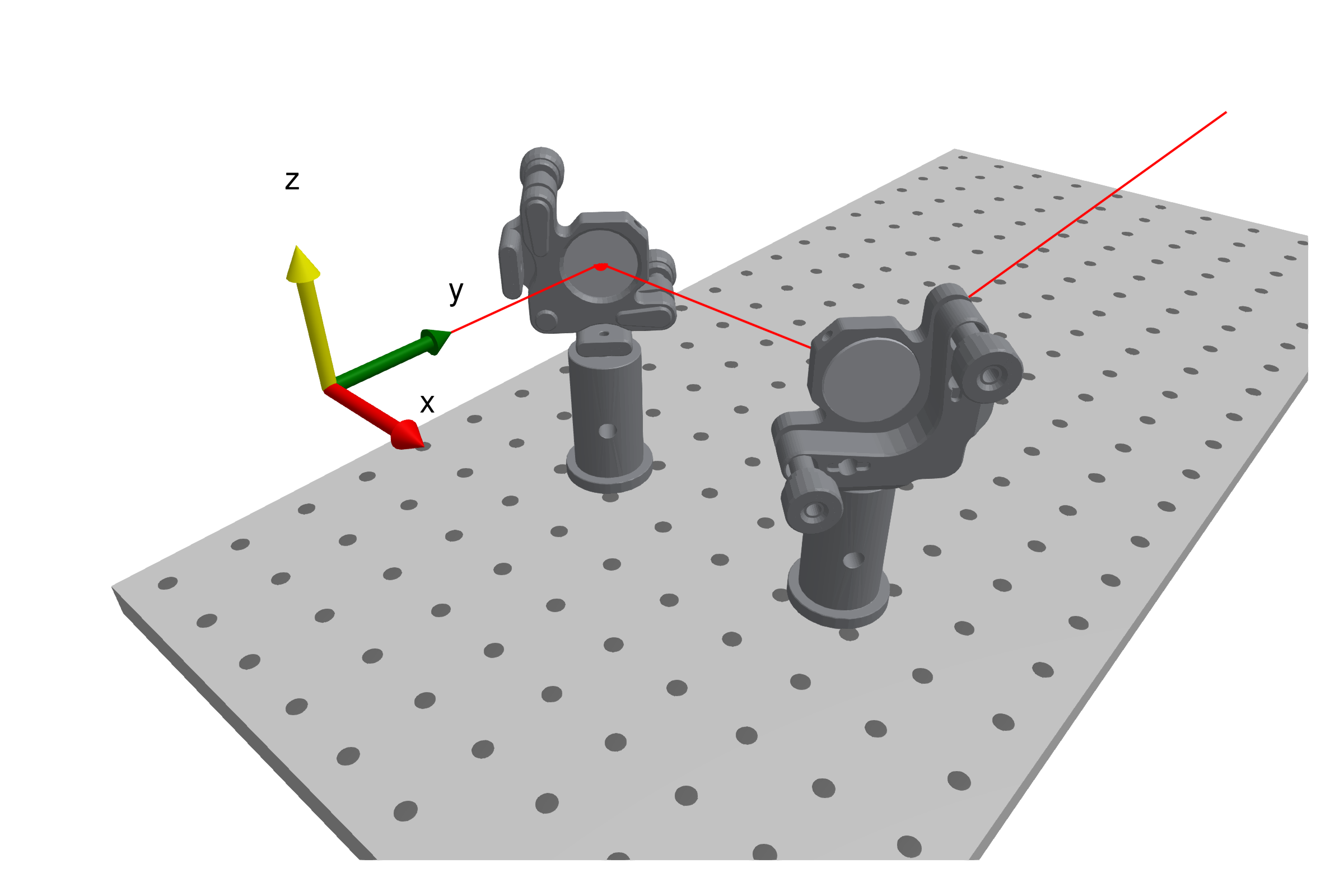

Finding the misalignment

In practice, mirror mounts are never perfectly aligned, and M1 has been knocked slightly out of place. We place an alignment card on the optical axis, 200 mm past M2, to see where the beam actually lands.

card = Detector(BMO.inch, false)       # alignment card: records hits, lets the beam pass
translate3d!(card, [Δx, 300mm, 0])
system = System([m1, m2, card])

function check_alignment()
    empty!(card)
    solve_system!(system, Beam(Ray([0, 0, 0], [0, 1.0, 0], λ)))
    offset = spot_diagram(card)[1]     # [x, z] on the card
    println("offset on card: x = ", round(offset[1] / mm, digits=4) + 0, " mm, z = ", round(offset[2] / mm, digits=4) + 0, " mm")
    return offset
end

offset = check_alignment()

2-element Point{2, Float64} with indices SOneTo(2):
 0.0038796811348679183
 0.001196571890907369

A Detector with stop = false behaves like a real alignment card: it records where the beam hits, but lets the beam continue propagating through the rest of the system rather than absorbing it. Detectors accumulate hits over successive calls to solve_system!, so check_alignment calls empty! first to discard any previous data. We will reuse it below to check our corrections.

To see the result, we plot the setup next to the card:

function plot_alignment()
    beam = Beam(Ray([0, 0, 0], [0, 1.0, 0], λ))
    solve_system!(system, beam)
    fig = Figure(size=(600, 400))
    ax = LScene(fig[1,1], show_axis=false)
    optical_table!(ax)
    render!(ax, system)
    render!(ax, beam, color=:red, flen=0.3, show_pos=true)
    spot_ax = Axis(fig[1,2], aspect=1, xlabel="x [mm]", ylabel="z [mm]",
        limits=(-12.7, 12.7, -12.7, 12.7), title="Card")
    scatter!(spot_ax, [0.0], [0.0], color=:black, marker=:xcross, markersize=16)
    pts = spot_diagram(card)
    scatter!(spot_ax, [p[1]/mm for p in pts], [p[2]/mm for p in pts], color=:red)
    return fig
end

fig2 = plot_alignment()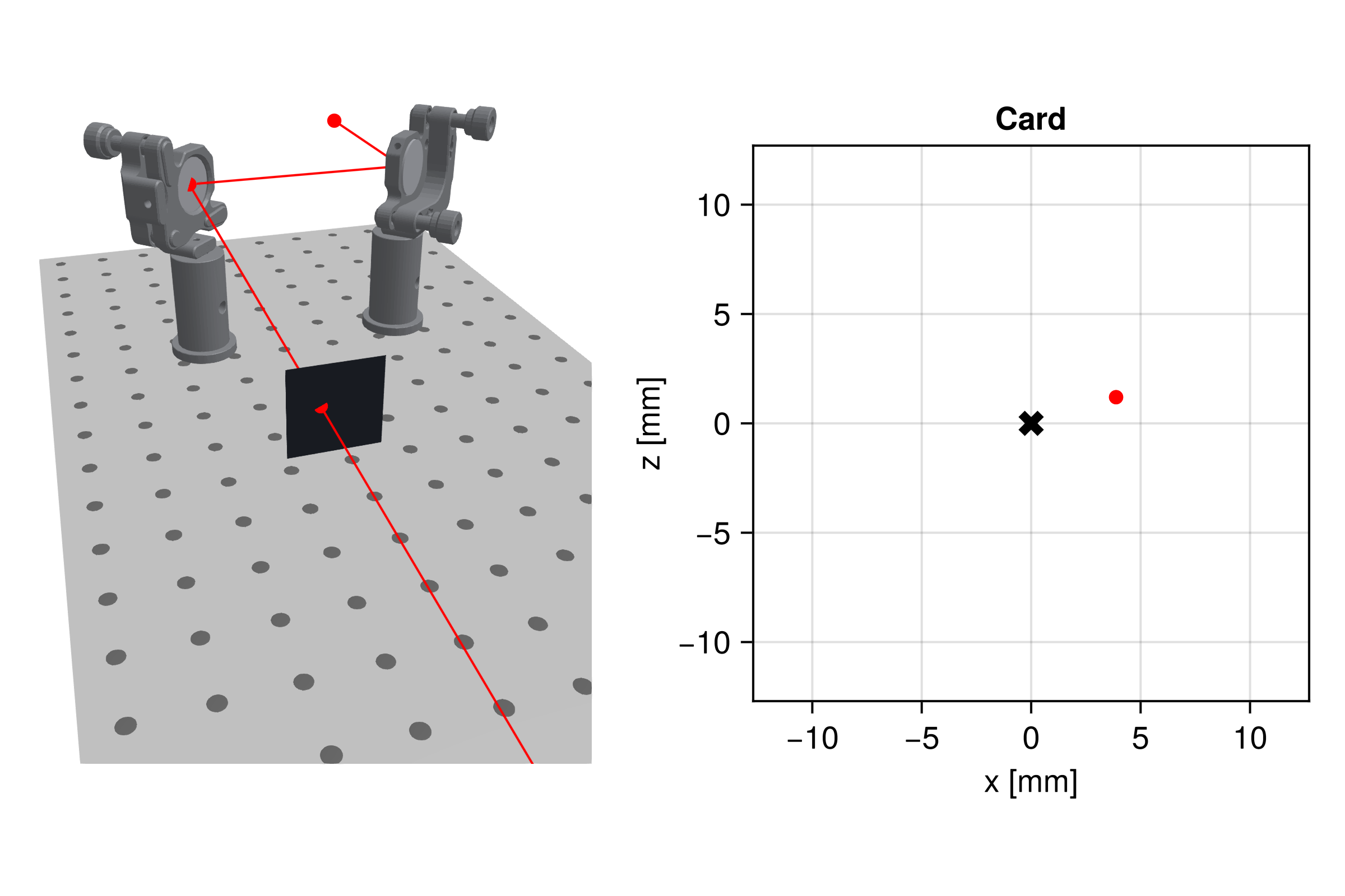

The black cross marks the intended target at the center of the card. The red dot shows where the beam actually lands: about 3.9 mm to the side and 1.2 mm up.

Correcting the mirror

Now it is your turn: bring the spot back to the center of the card by rotating M1 with zrotate3d! and xrotate3d!, just as you would turn the two adjustment screws of the mount. Two small-angle rules help to estimate the angles from the offset on the card, which sits a path length   mm behind M1 (across to M2, then along the axis to the card):

• Rotating M1 by about the vertical z-axis turns the reflected beam by within the table plane.

• Rotating M1 by about the global x-axis tilts it out of the plane of incidence. Because M1 sits at 45°, only part of this tilt acts on the beam, which is deflected vertically by just , not . A positive rotation moves the spot down.

Together, this gives

Solve these for the angles, rotate M1 back by them and call check_alignment() again. Since the rules are only approximate, a second iteration brings you closer still.

L = 300mm                              # M1 → M2 → card
# Your turn, e.g.:
# zrotate3d!(m1, ...)
# xrotate3d!(m1, ...)
# check_alignment()

0.3

Show solution

M1 was first rotated by −0.23° about the x-axis and then by +0.37° about the z-axis. Rotations do not commute, so we undo them in reverse order:

zrotate3d!(m1, deg2rad(-0.37))
xrotate3d!(m1, deg2rad(0.23))
check_alignment()

2-element Point{2, Float64} with indices SOneTo(2):
 -1.710181996017468e-10
 -3.3505726713062895e-19

The residual offset is far below a micrometer. Estimating the angles with the rules above gets you within about 10 µm on the first try.

With M1 corrected, the beam hits the center of the card and runs along the optical axis of the setup:

fig3 = plot_alignment()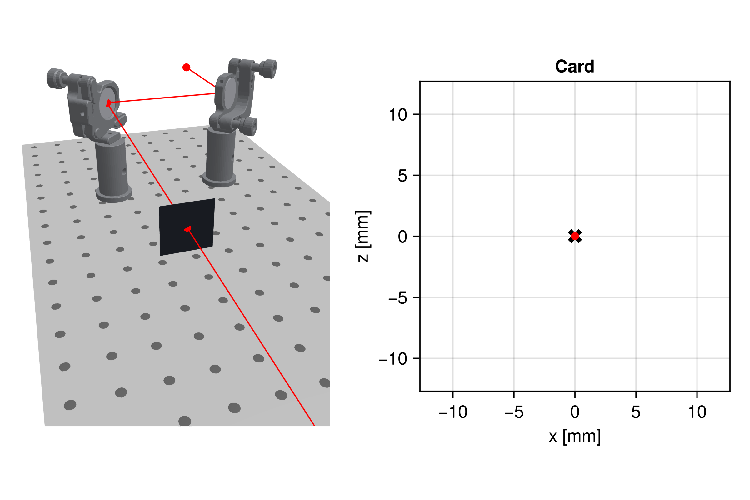

Next steps

From here, you could continue with the Michelson interferometer tutorial to see how a similar beam is split and recombined, the Miniature microscope tutorial for a more complex multi-lens system, or browse the Optical components and Visualization sections for more details on the building blocks used here.