Rendering Gaussian beamlets

Gaussian beamlets are drawn as the surface of their 1/e² intensity envelope. With show_beams = true, the chief, waist and divergence rays that generate the beamlet are drawn as well. Example renderings can be found in the Stigmatic beamlets and Astigmatic beamlets sections.

Stigmatic Gaussian beamlets

BeamletOptics.render! Method

render!(ax, gauss::GaussianBeamlet; kwargs...)

Render the 1/e² envelope of the GaussianBeamlet into the specified axis.

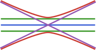
With show_beams = true the generating rays are overlayed into the axis as follows:

• chief beam: red

• divergence beam: green

• waist beam: blue

Keyword args

• show_beams = false: plot the generating rays of the GaussianBeamlet

• flen = 0.1: length of the final beam in case of no intersection

• r_res::Int = 50: radial resolution of the beam

• z_res::Int = 100: resolution along the optical axis of the beam

Makie kwargs

• color = :red

• transparency = true

Additional kwargs can be passed into the surface plot of the Gaussian envelope.

source

Astigmatic Gaussian beamlets

BeamletOptics.render! Method

render!(ax, agb::AstigmaticGaussianBeamlet; kwargs...)

Render the 1/e² envelope of the AstigmaticGaussianBeamlet as a smooth 3D surface.

With show_beams = true the generating rays are overlayed into the axis as follows:

• chief beam: red

• divergence beam: green

• waist beam: blue

Keyword args

• show_beams = false: plot the generating rays (chief, waist, divergence)

• flen = 0.1: length of the final beam segment in case of no intersection [m]

• z_res::Int = 100: longitudinal resolution

• r_res::Int = 64: radial (angular) resolution

Polarization kwargs

• show_polarization = false: overlay the E-field curve along the chief ray

• pol_λ = nothing: visualization wavelength [m], default = total plotted length / 20. This is a plotting parameter, not the physical ray wavelength; the curve shows the t = 0 snapshot Re{E⊥·exp(i·k·s)} along the accumulated optical path s. Gouy phase and phase-front curvature are ignored; the curve is a qualitative visualization only. Values finer than plotted length / 2000 are clamped with a warning.

• pol_scale = 1.0: curve amplitude as a multiple of the mean 1/e² beam radius at the start of the beamlet (at the maximum |E⊥|)

• pol_focus_exponent = 1.0: the amplitude follows the on-axis field amplitude, (A_ref / A(z))^(pol_focus_exponent/2) with A = wx·wy. 1 is the physical scaling E ∝ √(w0x·w0y / (wx·wy)), which raises the curve in the focus; values in (0, 1) compress the gain for tight foci, 0 gives a constant amplitude.

• pol_gain_max = 10.0: upper bound on the focus gain, in multiples of the reference amplitude at the start of the beamlet. The curve saturates at this value rather than leaving the scene when the beam focuses tighter downstream than its input waist.

• pol_ppl = 32: sample points per pol_λ along the curve

• pol_color = :crimson: field curve color

• pol_linewidth = 2.0: field curve line width

Makie kwargs

• color = :red

• transparency = true

source